Usually, measurement errors are reported as some multiple of the standard deviation: often the SD itself, or twice the SD, or occasionally some other multiple. To cover all these cases, let's just call that multiple $\kappa.$
In this fashion, taking the measurement errors to be independent, we may conceive of the numbers $x_i$ in your dataset as being of the form
$$x_i = y_i + \varepsilon_i$$
where the $y_i,$ $(i=1,2,\ldots, n)$ are the true underlying values modeled as a sample from a population or process with a distribution function $F,$ the $\sigma_i$ (when multiplied by $\kappa$) are the "plus or minus" values as given in the question, the $\varepsilon_i$ are independent random variables (and independent of the $y_i$) with variances $\sigma_i^2,$ and the $x_i$ are the measurements. Let's further assume the measurement method is unbiased: this means the expectations of the $\varepsilon_i$ are all zero.
Another assumption is needed: that the $\sigma_i$ are accurately known. (This often is not the case: the $\sigma_i$ often are just (fairly crude) estimates based on repeated measurements of each value. But sometimes the $\sigma_i$ are determined by a measurement system that has been calibrated and tested so often that its statistical properties are very well known and the $\sigma_i$ vary due to modifications of that system. For instance, the measurement error in a laboratory analysis of an aqueous concentration may depend on how much the sample was diluted during a preparation phase.)
With all these assumptions in place--the data are a sample from a distribution $F$ with mean $\mu$ and variance $\sigma^2;$ and their measurements are independent and unbiased with known standard deviations--we may estimate the mean with a formula like
$$\bar x = \sum_{i=1}^n \omega_i\,x_i = \sum_{i=1}^n \omega_i\left(y_i + \varepsilon_i\right)$$
where the $\omega_i$ are suitable positive numbers. To make them suitable, we need the expectation of $\bar x$ to equal the expectation of $F,$ which implies the $\omega_i$ must sum to unity; and among all such possible $\omega_i,$ we may select the ones that minimize the variance of $\bar x,$ given by
$$\operatorname{Var}(\bar x) = \operatorname{Var}\left(\sum_{i=1}^n \omega_i\left(y_i + \varepsilon_i\right)\right) = \sum_{i=1}^n \omega_i^2 \left(\sigma^2 + \sigma_i^2\right).$$
This is minimized when the $\omega_i$ are inversely proportional to the factors $\sigma^2 + \sigma_i^2.$ Choosing this solution gives
$$\bar x = \frac{\sum_{i=1}^n \frac{x_i}{\sigma^2 + \sigma_i^2}}{\sum_{i=1}^n \frac{1}{\sigma^2 + \sigma_i^2}};\quad \operatorname{Var}(\bar x) = \frac{\sum_{i=1}^n \frac{1}{\sigma^2 + \sigma_i^2}}{\left(\sum_{i=1}^n \frac{1}{\left(\sigma^2 + \sigma_i^2\right)}\right)^2}.$$
That's a correct answer, insofar as it goes: but we usually don't know the value of $\sigma^2.$ It needs to be estimated. That raises the question of how best to estimate it.
One reasonable (although not necessarily optimal) procedure is to estimate $\sigma$ and the weights iteratively. That is, given some estimate $\hat\sigma_j^2$ of $\sigma^2$ obtained after $j$ iterations, compute the weights
$$\omega_{i;j+1} = \frac{1}{\sum_{i=1}^n \frac{1}{\hat\sigma_j^2 + \sigma_i^2}}\left(\frac{1}{\hat\sigma_j^2 + \sigma_i^2}\right)$$
and with them update the estimated (weighted) mean
$$\bar x_{j+1} = \sum_{i=1}^n \omega_{i;j+1}\,x_i$$
and then update the estimate $\hat\sigma^2$ to a new value $\hat\sigma^2_{j+1}.$ Extensive simulations suggest a good update would be a bias-adjusted weighted variance from which the contributions of the $\sigma_i^2$ have been removed:
$$\hat\sigma^2_{j+1} = \frac{n}{n-1}\sum_{i=1}^n \omega_{i;j+1}(x_i - \bar x_{j+1})^2 - \frac{1}{n} \sum_{i=1}^n \sigma_i^2.$$
(This formula is inspired by the weights that are applied when there is no measurement error: in that case, they are all equal to $1/(n-1),$ which is $n/(n-1)$ times the weights $\omega_i = 1/n$ that would be used. Using values of $0$ for all the $\sigma_i$ will thereby cause the algorithm to converge immediately to the usual unbiased variance estimate.)
Whenever this value is negative, set it to zero. Iterate until the $\hat\sigma^2_j$ converge, as tested by comparing $\hat\sigma^2_{j+1} / \hat\sigma^2_j$ to $1.$
The iteration may begin by setting $\hat\sigma^2_0$ to be the naive (unweighted) variance estimate of the $x_i$ (computed by setting all weights to $1/n$).
This algorithm appears always to converge and to produce nearly unbiased estimates of $\sigma^2$ provided $\sigma^2$ is not close to the root mean square of the $\sigma_i^2.$ Specifically,
When the variation among the measured values $x_i$ can be explained by the measurement errors, $\sigma^2$ is likely small and often is estimated as $0.$
When the measurement errors are small compared to the variation among the measured values, this procedure estimates $\sigma^2$ accurately on average.
When the spread of the true values is comparable to the measurement errors, this procedure tends to underestimate $\sigma^2.$
Such behavior looks unavoidable in small datasets due to the difficulty of estimating $\sigma^2$ precisely even with zero measurement error.
For the data in the question, interpreting the $\pm$ values as standard deviations of the measurements (that is, $\kappa=1$), this procedure converges after three iterations (to a precision of one in a million) to the estimates $\bar x_3 = 9.167$ and $\hat\sigma_3^2 = 3.801.$ We may take $\hat \sigma = \sqrt{\hat\sigma_3^2} = 1.95.$ Because this exceeds most of the measurement standard deviations, it is probably an accurate estimate.
At the end the weights are
$$\omega = (\omega_{i;3}) = (0.2719, 0.2304, 0.2981, 0.1996).$$
As we expect, lower weights are associated with the measurements having greater error--but the variation in the weights is not great, given that the measurement SDs vary by a factor of three.
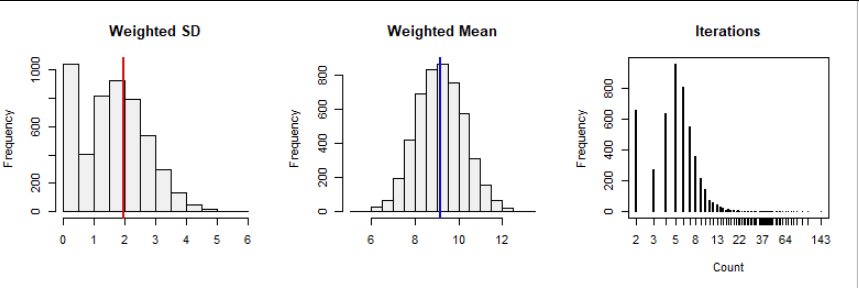
As a further test, I performed a parametric bootstrap, assuming the $y_i$ are sampled from a Normal distribution. This procedure drew 5,000 values of the $y_i$ from a Normal distribution having the same (weighted) mean and variance reported above, applied random measurement errors to those $y_i$ with the given standard deviations, and ran the proposed procedure to estimate the mean and variance of this Normal distribution. Here is a graphical summary of the results:

The vertical colored bars show the true underlying values in the bootstrap. They are positioned squarely in the middle of the bootstrap distributions of their estimates, indicating a lack of bias. The bar plot of iteration counts at the right indicates that few iterations were needed in the great majority of cases and often 2 - 5 iterations sufficed.
The spread of estimates of $\bar x$ indicates the error of the mean. The middle 95% of these values lie in the interval $[7.0, 11.3],$ for instance. We may communicate this by saying we are 95% confident the true mean (of the $y_i$) lies between $7.0$ and $11.3.$
To make the details perfectly clear, here is the R code implementing the variance estimation algorithm (as var.wt) and performing the parametric bootstrap.
#
# An iterative procedure to estimate mean and variance from a set of
# measurements `x` made with known measurement errors `sigma.i`.
#
var.wt <- function(x, sigma.i, thresh=1e-6, iter.max=200) {
  #
  # To avoid giving undue weight to any subset, all SDs should be nonzero.
  #
  if (missing(sigma.i)) sigma.i <- rep(0, length(x)) # No measurement error
  tol <- sum(abs(x)) * 1e-16
  sigma.i[sigma.i <= 0] <- min(c(tol, sigma.i[sigma.i > 0])) / 2
  #
  # Initialize.
  #
  v <- var(x)
  n <- length(x)
  S <- mean(sigma.i^2) # Avoids recomputing this constant within the loop
  for (i in 1:iter.max) {
    w <- 1/(v + sigma.i^2); w <- w / sum(w)
    m <- sum(x * w)
    v.0 <- max(0, sum((x-m)^2 * w) * n / (n-1) - S)
    if (v <= v.0 * (1+thresh) && v.0 <= v * (1+thresh)) break
    v <- v.0
  }
  if (i >= iter.max) warning("Maximum iteration count exceeded.")
  list(Variance=v, Mean=m, Iterations=i)
}
#
# The data in the question.
#
x <- c(10, 12, 7, 8)
sigma.i <- c(0.8, 1.2, 0.5, 1.5)
(s <- var.wt(x, sigma.i))
#
# A parametric bootstrap.
#
n <- length(x)
sigma <- sqrt(s$Variance)
mu <- s$Mean
set.seed(17)
X <- replicate(5e3, {
  y <- rnorm(n, mu, sigma)
  epsilon <- rnorm(n, 0, sigma.i)
  x <- y + epsilon
  var.wt(x, sigma.i)
})
X <- matrix(unlist(X), 3)
#
# Display the results.
#
par(mfrow=c(1,3))
hist(sqrt(X[1,]), main="Weighted SD", col="#f0f0f0", xlab="")
abline(v = sigma, lwd=2, col="#d01010")
hist(X[2,], main="Weighted Mean", col="#f0f0f0", xlab="")
abline(v = mu, lwd=2, col="#1010d0")
plot(table(X[3,]), log="x", main="Iterations", xlab="Count", ylab="Frequency")
par(mfrow=c(1,1))

(quantile(X[2,], c (0.025, 0.975))) # A central 95% interval of the weighted means


