Mixed model for repeated measures data using lme4/lmer in R

Question

I'd appreciate some advice specifying a mixed effects model using the lme4 package in R.

I have pre/post measurements for approximately a thousand schoolchildren, clustered within schools. 30 of the schools received an intervention to encourage the children to be more physically active. The other schools were controls. Minutes per day spent physically active by each child were recorded at both time points (wave 1 and 2) using an accelerometer worn for 7 days. The intervention and control groups were equally active at the first time point. The data structure looks like:

> str(activity_data)
Classes ‘tbl_df’, ‘tbl’ and 'data.frame':   1532 obs. of  6 variables:
 $ id               : num  2 2 3 3 4 4 5 5 8 8 ...
 $ school           : Factor w/ 61 levels "1","2","3","4",..: 1 1 1 1 1 1 1 1 1 1 ...
 $ intervention     : Factor w/ 2 levels "0","1": 1 1 1 1 1 1 1 1 1 1 ...
 $ wave             : Factor w/ 2 levels "0","1": 1 2 1 2 1 2 1 2 1 2 ...
 $ minutes_active   : int  212 219 210 211 246 166 145 152 257 236 ...
 $ monitor_wear_time: int  774 741 718 778 876 850 727 766 807 881 ...

I am trying to determine whether there is a difference in time spent physically active at the second time point between the intervention and control groups. From reading other posts on SE, I believe that there are 3 levels in my model: 1) wave, 2) id, 3) school.

lmer_fit <- lmer(minutes_active ~ intervention * wave + monitor_wear_time + (1 | id) + (1 | school),
                   data = activity_data)

A) Is this model appropriate given the data structure and the question I am trying to answer?

B) I have included monitor_wear_time in the model to account for the fact that the time recorded as being physically active is dependent on how much time a child actually wears the activity monitor. Is simply including it as a covariate an appropriate way to achieve this?

Working through a solution based on Erik's answer

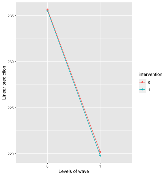
Eyeballing the fixed effects of the lmer_fit model and having fitted it using lmerTest::lmer to provide p-values, the output suggests that there is a decline in activity of approximately 15 minutes between baseline and follow-up, whereas being in the intervention group seems to have little effect. How long a child wears the monitor does seem to be associated with minutes spent active, as would be expected.

Fixed effects:
                      Estimate Std. Error         df t value Pr(>|t|)    
(Intercept)          -10.54322   11.35297 1327.72296  -0.929    0.353    
intervention1         -0.11718    3.52698   55.56354  -0.033    0.974    
wave1                -15.45528    1.50644  767.20177 -10.260   <2e-16 ***
monitor_wear_time      0.31390    0.01424 1327.44860  22.044   <2e-16 ***
intervention1:wave1   -0.28823    2.00013  765.56199  -0.144    0.885   

Using emmeans::emmip(lmer_fit, intervention ~ wave) to plot minutes active against wave for both groups suggests there is little difference in marginal means between the two groups at either baseline or follow-up. However, it does suggest that activity declined by roughly the same amount in both groups over time:

Finally, using emmeans::emmeans(lmer_fit, pairwise ~ intervention | wave) performs two contrasts — comparing the marginal means for minutes active between the two groups at each time point separately. If I've understood 'marginal means' correctly, in this example it is comparing the mean minutes active between the two groups having adjusted for the other covariates specified in the lmer_fit model (id, school, monitor wear time).

emm1 <- emmeans::emmeans(lmer_fit, pairwise ~ intervention | wave)
emm1$contrasts %>% confint() %>% as.data.frame()
  contrast wave  estimate       SE       df  lower.CL upper.CL
1    0 - 1    0 0.1171780 3.534990 61.06601 -6.951317 7.185673
2    0 - 1    1 0.4054121 3.531597 60.87412 -6.656748 7.467572

Judging by the confidence intervals, there appears to be little difference between the marginal means of minutes active between the intervention and control groups at either time point.

Please correct me if I've misunderstood anything or suggest a better answer

Answer 1

From reading other posts on SE, I believe that there are 3 levels in my model: 1) wave, 2) id, 3) school.

Absolutely this is the case and your model code reflects this structure and would even account for the possibility of a student who being observed in more than 1 school.

I am trying to determine whether there is a difference in time spent physically active at the second time point between the intervention and control groups.

This is going to require a little bit of work to answer. Your current model with an intervention * wave interaction is a start, but will give you different information. First, let me suggest that you recode wave 1 to be 0 and wave 2 to be 1. These models make more sense when categorical variables have a valid 0 variable. This is easily done in dplyr:

library(dplyr)
activity_data <- activity_data %>% recode(wave, `1` = 0L, `2` = 1L) 

Once you do this, your intervention * wave interaction will test whether the intervention effect is greater at wave 2 vs wave 1. But what you want to know is whether the intervention effect is significant at wave 2 itself, not whether it is greater at wave 2 relative to wave 1.

For that, you have multiple options. Perhaps the simplest is to run the pairwise comparisons after you have run the model:

library(emmeans)
#graph
emmip(lmer_fit, type ~ intervention | wave)
#tests
emmeans(lmer_fit, pairwise ~ intervention)

This code should work, but might have to be massaged a bit.

Answer 2

I'm guessing what you want to do then is perform a test to find out if there is a statistical difference between the two groups, correct?

You probably want to make sure you try different model specifications - look at section 4.4: http://sia.webpopix.org/lme.html. It is appropriate to include monitor_wear_time as a covariate as you did. You might want to plot that covariate according to the treatment variable and according to the target variable - this will give you an idea of how likely it is to be correlated with the respective variables.

Regarding the hypothesis testing, if you only have 30 schools you may run into problems of sample size and degrees of freedom (the latter depending on the model specification you opt for in the first place). Maybe this can help: https://www.ssc.wisc.edu/sscc/pubs/MM/MM_TestEffects.html

In the end something like a Wald test or likelihood ratio should be satisfactory but tough to say without looking at it in more detail.

I believe mixed models can help with your setup but it's not the only one, however! Have you thought at whether looking into a simple paired t-test could yield any insight? Paired t-test as a special case of linear mixed-effect modeling