64
$\begingroup$

I have a random sample of Bernoulli random variables $X_1 ... X_N$, where $X_i$ are i.i.d. r.v. and $P(X_i = 1) = p$, and $p$ is an unknown parameter.

Obviously, one can find an estimate for $p$: $\hat{p}:=(X_1+\dots+X_N)/N$.

My question is how can I build a confidence interval for $p$?

$\endgroup$
1

4 Answers 4

68
$\begingroup$
  • If the average, $\hat{p}$, is not near $1$ or $0$, and sample size $n$ is sufficiently large (i.e. $n\hat{p}>5$ and $n(1-\hat{p})>5$, the confidence interval can be estimated by a normal distribution and the confidence interval constructed thus:

    $$\hat{p}\pm z_{1-\alpha/2}\sqrt{\frac{\hat{p}(1-\hat{p})}{n}}$$

  • If $\hat{p} = 0$ and $n>30$, the $95\%$ confidence interval is approximately $[0,\frac{3}{n}]$ (Javanovic and Levy, 1997); the opposite holds for $\hat{p}=1$. The reference also discusses using using $n+1$ and $n+b$ (the later to incorporate prior information).

  • Else Wikipedia provides a good overview and points to Agresti and Couli (1998) and Ross (2003) for details about the use of estimates other than the normal approximation, the Wilson score, Clopper-Pearson, or Agresti-Coull intervals. These can be more accurate when above assumptions about $n$ and $\hat{p}$ are not met.

R provides functions binconf {Hmisc} and binom.confint {binom} which can be used in the following manner:

set.seed(0)
p <- runif(1,0,1)
X <- sample(c(0,1), size = 100, replace = TRUE, prob = c(1-p, p))
library(Hmisc)
binconf(sum(X), length(X), alpha = 0.05, method = 'all')
library(binom)
binom.confint(sum(X), length(X), conf.level = 0.95, method = 'all')

Agresti, Alan; Coull, Brent A. (1998). "Approximate is better than 'exact' for interval estimation of binomial proportions". The American Statistician 52: 119–126.

Jovanovic, B. D. and P. S. Levy, 1997. A Look at the Rule of Three. The American Statistician Vol. 51, No. 2, pp. 137-139

Ross, T. D. (2003). "Accurate confidence intervals for binomial proportion and Poisson rate estimation". Computers in Biology and Medicine 33: 509–531.

$\endgroup$
8
  • 5
    $\begingroup$ (+1) Nice answer. This will become a reference for similar questions in the future, I think. However, cross-posting is unusual; in fact, I believe it is frowned on, because it screws up many aspects of the feedback/referencing/threading/commenting system. Please consider removing one of the copies and replacing it by a link in a comment. $\endgroup$
    – whuber
    Commented Jan 12, 2011 at 2:49
  • $\begingroup$ @whuber thanks for the feedback. I have removed the other copy. $\endgroup$ Commented Jan 12, 2011 at 2:53
  • $\begingroup$ In the first formula, what are z1 and alpha? $\endgroup$
    – Cirdec
    Commented Nov 22, 2013 at 17:44
  • $\begingroup$ I found the answer to my own question: $z_{1-\alpha/2}$ is the ${1-\alpha/2}$ percentile of the standard normal distribution and $\alpha$ is the error percentile. en.wikipedia.org/wiki/Binomial_proportion_confidence_interval $\endgroup$
    – Cirdec
    Commented Nov 22, 2013 at 17:50
  • 2
    $\begingroup$ Why not simply using binom.test() in R which implements the Clopper-Pearson method? $\endgroup$
    – rnorouzian
    Commented Dec 20, 2017 at 15:34
14
$\begingroup$

Maximum likelihood confidence intervals

The normal approximation to the Bernoulli sample relies on having a relatively large sample size and sample proportions far from the tails. The maximum likelihood estimate focuses on the log-transformed odds and this provides non-symmetric, efficient intervals for $p$ that should be used instead.

Define the log-odds as $\hat{\beta}_0 = \log(\hat{p}/(1-\hat{p}))$

A 1-$\alpha$ CI for $\beta_0$ is given by:

$$\text{CI}(\beta_0)_\alpha = \hat{\beta}_0 \pm \mathcal{Z}_{\alpha/2} \sqrt{1/(n\hat{p}(1-\hat{p})}$$

And this is back transformed into a (non-symmetric) interval for $p$ with:

$$\text{CI}(p)_\alpha = 1/(1+\exp(-\text{CI}(\beta_0)_\alpha)$$

This CI has the added benefit that proportions lie in the interval between 0 or 1, and the CI is always narrower than the normal interval while being of the correct level. You can get this very easily in R by specifying:

set.seed(123)
y <- rbinom(100, 1, 0.35)
plogis(confint(glm(y ~ 1, family=binomial)))

    2.5 %    97.5 % 
0.2795322 0.4670450 

Exact binomial confidence intervals

In small samples, the normal approximation to the MLE--while better than the normal approximation to the sample proportion--may not be reliable. That is okay. $Y = n\hat{p}$ can be taken to follow a binomial$(n,p)$ density. Bounds for $\hat{p}$ can be found taking the 2.5th and 97.5-th percentiles from this distribution.

$$\text{CI}_\alpha = (F^{-1}_{\hat{p}}(0.025), F^{-1}_{\hat{p}}(0.975))$$

Rarely possible by-hand, an exact binomial confidence interval can be obtained for $p$ using computational methods.

qbinom(p = c(0.025, 0.975), size = length(y), prob = mean(y))/length(y)
[1] 0.28 0.47

Median unbiased confidence intervals

And if $p$ is 0 or 1 exactly, a median unbiased estimator can be used to obtain non-singular interval estimates based on the median unbiased probability function. You can trivially take the lower bound of the all-0 case as 0 WLOG. The upper bound is any proportion $p_{1-\alpha/2}$ that satisfies:

$$p_{1-\alpha/2} : P(Y = 0)/2 + P(Y > y) > 0.975$$

This is also a computational routine.

set.seed(12345)
y <- rbinom(100, 1, 0.01) ## all 0
cil <- 0
mupfun <- function(p) {
  0.5*dbinom(0, 100, p) + 
    pbinom(1, 100, p, lower.tail = F) - 
    0.975
} ## for y=0 successes out of n=100 trials
ciu <- uniroot(mupfun, c(0, 1))$root
c(cil, ciu)

[1] 0.00000000 0.05357998 ## includes the 0.01 actual probability

The last two methods are implemented in the epitools package in R.

$\endgroup$
1
  • 1
    $\begingroup$ For reference: I believe the last type of confidence interval (median unbiased ci) is also called (Clopper-Pearson) mid-P confidence interval (see Agresti & Gottard (2005)). $\endgroup$ Commented Feb 15, 2022 at 20:04
2
$\begingroup$

The Wilson score interval performs well in general for inference for the binomial probability parameter. The performance of various confidence intervals is examined in Brown, Cai and DasGupta (2001) and the Wilson score interval performs well compared to other intervals; in particular, it performs better than the Wald interval. The Wilson score interval has a number of useful consistency properties and it can be extended to handle both finite and infinite populations (see O'Neill 2021 for details).

The Wilson score interval can be implemented for finite or infinite populations in R using the CONF.prop function in the stat.extend package. In the code below we give a simple example of a 95% confidence interval for the probability parameter for an infinite superpopulation. To obtain a confidence interval for the proportion quantity in a finite population (either the full population or the unsampled part) you can add inputs for the population size N and the logical value unsampled.

#Set parameters
n <- 40
p <- 0.15

#Generate some binary data
set.seed(1)
x <- sample(c(0,1), size = n, replace = TRUE, prob = c(1-p, p))

#Generate a 95% confidence interval for probability parameter
library(stat.extend)
CONF.prop(x, alpha = 0.05)

        Confidence Interval (CI) 
 
95.00% CI for proportion parameter for infinite population 
Interval uses 40 binary data points from data x with sample proportion = 0.1500 

[0.0706118771732036, 0.290723243664897]
$\endgroup$
0
$\begingroup$

Suppose $X_1,...,X_n$ is a sample of successes and failures from a Bernoulli population with probability of success $p$, and we are asked to find a 75% confidence interval for $p$.

One solution is to invert the CDF of a binomial distribution. Since $Y=\sum X_i\sim \text{Binomial}(n,p)$ we can define a $100(1-\alpha)\%$ confidence interval for $p$ as $$\bigg\{p:F_Y(y;n,p)\ge\alpha/2 \text{ and } 1-F_Y(y-1;n,p)\ge\alpha/2 \bigg\}$$ where $F_Y(y;n,p)=P(Y\le y)$ is the CDF of $Y$.

An approximate solution is to note that $\text{Var}[\sum X_i]=np(1-p)\implies\text{Var}[\bar{X}]=p(1-p)/n$, where $\bar{X}=\frac{1}{n}\sum X_i$, and construct a $100(1-\alpha)\%$ confidence interval for $p$ by inverting a Wald test $$\bigg\{p: \Phi\bigg(\frac{\bar{x}-p}{\bar{x}(1-\bar{x})}\bigg)\ge \alpha/2 \text{ and } 1-\Phi\bigg(\frac{\bar{x}-p}{\bar{x}(1-\bar{x})}\bigg)\ge \alpha/2\bigg\}$$ $$= \bar{x}\pm z_{1-\alpha/2}\hat{\text{se}}$$ where $\hat{\text{se}}=\sqrt{\bar{x}(1-\bar{x})/n}$, $\Phi(\cdot)$ is the CDF of a standard normal distribution, and $z_{1-\alpha/2}$ is the $(1-\alpha/2)^{th}$ percentile of the standard normal distribution. The Wald test approximates the binomial sampling distribution of $\sum X_i$, or equivalently the distribution of $\bar{X}$, using a normal distribution and expresses it in terms of the standard normal CDF.

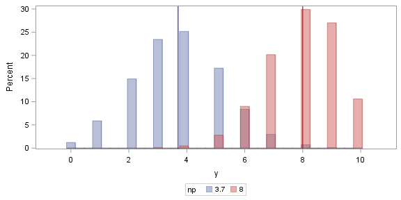
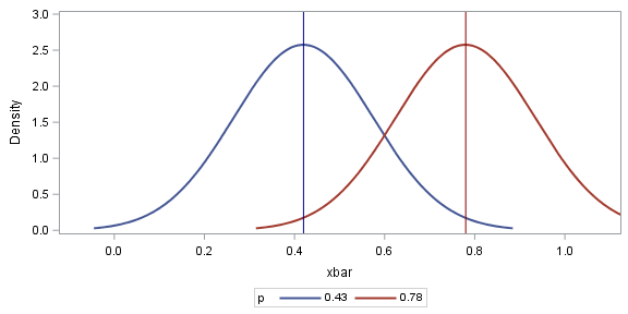
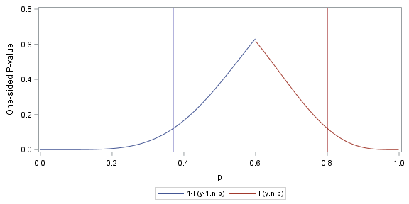
For example, if you observed $y=\sum x_i=6$ out of $n=10$ trials, $\bar{x}=0.6$. The $75\%$ confidence interval from inverting the binomial CDF is (0.37, 0.8). If $p$ is truly $0.37$ we would observe a result as or more extreme than $\bar{x}=0.6$ only $12.5\%$ of the time. Likewise, if $p$ is truly $0.8$ then $12.5\%$ of the time would we would observe a result as or more extreme than $\bar{x}=0.6$. In this way we are $75\%$ confident that the unknown fixed true $p$ is in $(0.37, 0.8)$. Intervals constructed in this manner will cover the unknown fixed true $p$ $75\%$ of the time in repeated sampling, and ours is one such sample. The confidence interval from inverting a Wald test is (0.42, 0.78).

$$\text{Inverting Binomial Sampling Distribution CDF} $$ $$\text{(PMF Depicted Below)}$$ enter image description here

enter image description here

$$\text{Inverting Normal CDF Approximating X-bar Sampling Distribution} $$ $$\text{(Normal Density Depicted Below)}$$ enter image description here

$$\text{One-sided P-value from Inverting Binomial CDF} $$ enter image description here

The confidence curve above shows p-values and confidence intervals of all levels from inverting the binomial CDF.

$\endgroup$

Your Answer

By clicking “Post Your Answer”, you agree to our terms of service and acknowledge you have read our privacy policy.