MLE for $\sigma^2$ in $\mathcal{N}(\mathbf{Bz}, \mathbf{WW}^{\top} + \sigma^2 \mathbf{I})$

Question

I'm trying to compute the MLE of $\sigma^2$ in the model,

$$ \mathbf{x} \mid \mathbf{z} \sim \mathcal{N}(\mathbf{Bz}, \mathbf{WW}^{\top} + \sigma^2 \mathbf{I}). $$

Here, $\mathbf{x} \in \mathbb{R}^P$, $\mathbf{z} \in \mathbb{R}^K$, $\mathbf{B} \in \mathbb{R}^{P \times K}$, and $\mathbf{W}^{P \times K}$. In other words, I want to take the derivative of the log likelihood, set it equal to zero, and solve for $\sigma^2$

If the covariance matrix were just $\sigma^2 \mathbf{I}$, then the MLE would just be what you'd get for probabilistic PCA. However, this log likelihood has the following term:

$$ (\mathbf{WW}^{\top} + \sigma^2 \mathbf{I})^{-1}. $$

I don't know how to either compute the derivative of this term w.r.t. to $\sigma^2$ or even how to isolate $\sigma^2$, since the Woodbury matrix formula will keep $\sigma^2$ inside the inverse.

Answer 1

I'll use $\tau = \sigma^2$ for simpler notation so we have $$ x\mid z\sim\mathcal N(Bz, WW^T + \tau I). $$ The (conditional) log likelihood is $$ \ell(\sigma\mid x,z) = -\frac 12 (x-Bz)^T(WW^T + \tau I)^{-1}(x-Bz)- \log\det(WW^T + \tau I). $$

Setting $r = x - Bz$, I can now use the fact that $WW^T$ is square, symmetric, and nonrandom to diagonalize it as $WW^T = Q\Lambda Q^T$. Then $$ \ell = -\frac12 r^TQ(\Lambda+\tau I)^{-1}Q^Tr - \log\det (\Lambda+\tau I) \\ = -\frac 12 u^T(\Lambda+\tau I)^{-1}u - \log\det (\Lambda+\tau I) \\ = -\frac 12 \sum_{i=1}^n \frac{u_i^2}{\lambda_i + \tau} - \sum_{i=1}^n \log(\lambda_i + \tau) $$ where I've used $u = Q^Tr$.

Taking the derivative w.r.t. $\tau$ I get $$ \ell' = \frac 12 \sum_i \frac{u_i^2}{(\lambda_i + \tau)^2} - \sum_i \frac 1{\lambda_i + \tau} \\ = \frac 12 u^T(\Lambda + \tau I)^{-2}u - \text{tr}(\Lambda + \tau I)^{-1} $$ if I want to write this in matrix form (I could have also used matrix calculus to get here directly).

I don't think we can analytically solve for this in general so numerical optimization will be the move.

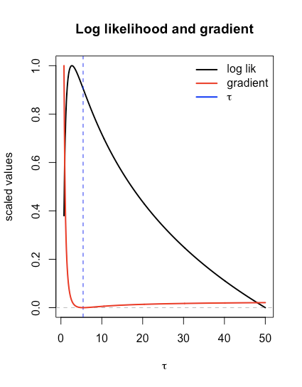
Here's an example comparing the likelihood to the gradient to check that it looks right.

set.seed(132)
n <- 35; p <- 8; m <- 11
B <- matrix(rnorm(m*n), n, m)
W <- matrix(rnorm(n*p), n, p)
z <- rnorm(m)
WWt <- W %*% t(W)
eig <- eigen(WWt)
tau <- 5.43
x <- MASS::mvrnorm(1, B %*% z, WWt + tau * diag(n))
u <- t(eig$vectors) %*% (x - B %*% z)

scale01 <- function(v) (v - min(v)) / (max(v) - min(v))  # for plotting

loglik <- Vectorize(function(tau) {
  -.5 * sum(u^2 / (eig$values + tau)) - sum(log(eig$values + tau))
})
gradloglik <- Vectorize(function(tau) {
  .5 * sum(u^2 / (eig$values + tau)^2) - sum(1 / (eig$values + tau))
})

curve(scale01(loglik(x)), .75, 50, 500, lwd=2, xlab=bquote(tau),
      ylab="scaled values", main = "Log likelihood and gradient")
abline(h = 0, col="grey", lty=2)
abline(v = tau, col="blue", lty=2)
curve(scale01(gradloglik(x)), .75, 50, 500, add=TRUE, col="red", lwd=2)
legend("topright", bty="n", col=c(1,2,4), lwd=2, legend=c("log lik", "gradient", expression(tau)))