Normal distributed random numbers in time - expected behaviour - askew distributions?

Question

I have a 3D array of numbers, initialised with normal distributed values. The mean of the distribution is $0$, the standard deviation in the order of $10^{-5}$ to $10^{-8}$, but would be constant for the entire array and all time steps. The array is large enough to see that the introduced standard deviation and mean are there.

Before the next time step, the array gets relaxed (converges to the average of the field, that gets introduced by another force), but does not fully reach it. If it did, the distribution (minus the average of the field) would get the normal distribution again and I would reach the previous state again, with a slight shift. The average would for example be gravity, a force acting equally on the entire array (simply adding $+10^{-6}$ to every number, every timestep) and later something a little more complicated, but still a shift that could be resolved locally, by comparing to the almost identical surrounding numbers. The biggest difference to the surrounding would be the fluctuations, due to the mentioned normal distributed random.

The opposite would be no relaxation, so the normal distributions sum up over time. Since I am somewhere in between: What would the analytical solution of the time averaged normal distributed randoms be?

Could there be an influence of the average of the field? What would it be? Am I right in expecting the distribution to be askew, if the field did not fully relax?

(Over)simplified idea:

I will implement this in 3D, but since that does not change the problem I tried to simplify the example.

first scenario, full relaxation

Normal distributed random numbers $\Rightarrow$ add force $\Rightarrow$ set to mean $\Rightarrow$ add more normal distributed random numbers

$$ \overbrace{\begin{array}% 0.2&0.3&0.1\\ -0.4&0.1&0.3\\ 0.5&0.0&-0.2 \end{array}}^\text{random numbers} \Rightarrow \overbrace{\begin{array}% 1.2&1.3&1.1\\ 0.6&1.1&1.3\\ 1.5&1.0&0.8 \end{array}}^\text{added force/offset=1} \Rightarrow \overbrace{\begin{array}% 1.0&1.0&1.0\\ 1.0&1.0&1.0\\ 1.0&1.0&1.0 \end{array}}^\text{full relaxing} \Rightarrow \overbrace{\begin{array}% 0.8&1.2&1.0\\ 0.4&1.3&1.1\\ 1.4&1.1&0.7 \end{array}}^\text{added further random} $$

second scenario, no relaxation

Normal distributed random numbers $\Rightarrow$ add force $\Rightarrow$ add more normal distributed random numbers

$$ \overbrace{\begin{array}% 0.2&0.3&0.1\\ -0.4&0.1&0.3\\ 0.5&0.0&-0.2 \end{array}}^\text{random numbers} \Rightarrow \overbrace{\begin{array}% 1.2&1.3&1.1\\ 0.6&1.1&1.3\\ 1.5&1.0&0.8 \end{array}}^\text{added force/offset=1} \Rightarrow \overbrace{\begin{array}% 0.8&1.2&1.0\\ 0.4&1.3&1.1\\ 1.4&1.1&0.7 \end{array}}^\text{added further random} $$

But basically the idea is, in the second case I sum up randomly distributed variables, so this would not result in the same standard deviation, right? Also, the mean one of these variables would be $\neq 0$, therefore resulting in an askew distribution in the last array. Or would they really be as equal as I wrote in my oversimplified example?

The added force would (for now) be a constant and the added random would be normal distributed randoms with $0$ mean, different at each site. This could result in the same distribution (not necessarily the same numbers as above), but will it really be equal over several iterations?

Answer 1

This is a random walk with drift.

Each step in the first scenario goes through two stages. Initially, there is an array of zeros. Because there appears to be no use of the geometry of the array, we may think of this simply as a (fixed-length) vector of values.

Stage 1: Add independent Gaussian values to each entry of the vector.

Stage 2: Project the vector onto the vector of its mean values.

If we inspect the state only after Stage 2 each time, we have no need to look at the entire vector: a single component will do, because all components are the same. This component is obtained as the value from the previous step plus the mean of the values added at Stage 1. But that mean--as is well known--is itself Gaussian, with expectation and variance easily computed from the properties of the Gaussians in Stage 1. Thus, writing $x_t$ for the (common) value of all the vector components after Stage 2 in step $t$, we find that

$$x_{t+1} = x_{t} + \varepsilon_t$$

where $\varepsilon_t$ are iid Gaussian (with, say, common variance $\sigma^2$): that's the random walk. When the mean $\mu$ of these $\varepsilon_t$ is nonzero, it's a random walk with drift, but that's easily reduced to a random walk because then

$$x_{t+1} = (t+1)\mu + y_{t+1}; \quad y_{t+1} = y_t + \delta_t $$

with $\delta_t = \varepsilon_t + \mu$ having zero mean.

Understanding this, it's easy to characterize the process after Stage 1 of step $t+1$: the vector looks like

$$(y_{t,1}, y_{t,2}, \ldots) = (x_t + \gamma_{t,1}, x_t + \gamma_{t,2}, \ldots)$$

where the $\gamma_{t,i}$ are the independent Gaussians added at that stage. We now have all the information needed to compute properties of this process:

$$E[y_{t,i}] = E[x_t + \gamma_{t,i}] = E[x_t] + E[\gamma_{t,i}] = (t-1)\mu + E[\gamma_{t,i}].$$

$$\text{Var}(y_{t,i}) = \text{Var}(x_t + \gamma_{t,i}) = \text{Var}(x_t) + \text{Var}(\gamma_{t,i}) = (t-1)\sigma^2 + \text{Var}(\gamma_{t,i}).$$

Now let $i \ne j$:

$$\text{Cov}(y_{t,i}, y_{t,j}) = \text{Cov}(x_t + \gamma_{t,i}, x_t + \gamma_{t,j}) = (t-1)\sigma^2$$

For the general covariance calculation we exploit the symmetry of covariance and assume $s \gt t$. Recall that $x_s$ is obtained from $x_t$ by adding random variates independent of $x_t$, whence $\text{Cov}(x_s, x_t) = \text{Var}(x_t)$. Let the size of the array be $n$ and note that one (additive) component of $x_s$ is $\gamma_{t,i}/n$; besides this, the only things $x_s$ and $x_t$ have in common are $x_t$ itself. (That is, $x_s - (x_t + \gamma_{t,i})$ is the sum of variates independent of both $x_t$ and $\gamma_{t,i}$.) Thus

$$\text{Cov}(y_{t,i}, y_{s,j}) = \text{Cov}(x_t + \gamma_{t,i}, x_s + \gamma_{s,j}) = (t-1)\sigma^2 + \text{Var}(\gamma_{t,i})/n^2.$$

By virtue of Kolmogorov's Extension Theorem and the fact that multivariate Gaussian distributions are completely determined by their means and covariance matrices--which we have just fully computed--this is a complete characterization of the first scenario.

The second scenario (no relaxation) is simpler: each component of the vector independently is a random walk with drift.

This exposition has not assumed that the random variates added to the components have a common mean or common variance. Moreover, the calculations can be generalized so that all the random ingredients of the process have arbitrary means and variances, potentially varying from one point to another and from one step to another. This complicates the notation somewhat but the result is essentially the same (a random walk with drift and possible heteroscedasticity).

Similar calculations can be applied when the relaxation is performed on local neighborhoods of a grid. The computations of covariances become more complicated, because now we have to account for the geometric structure of the grid, but there are no new ideas introduced. The upshot is that you obtain a collection of correlated heteroscedastic random walks with drift, one per grid cell.

---

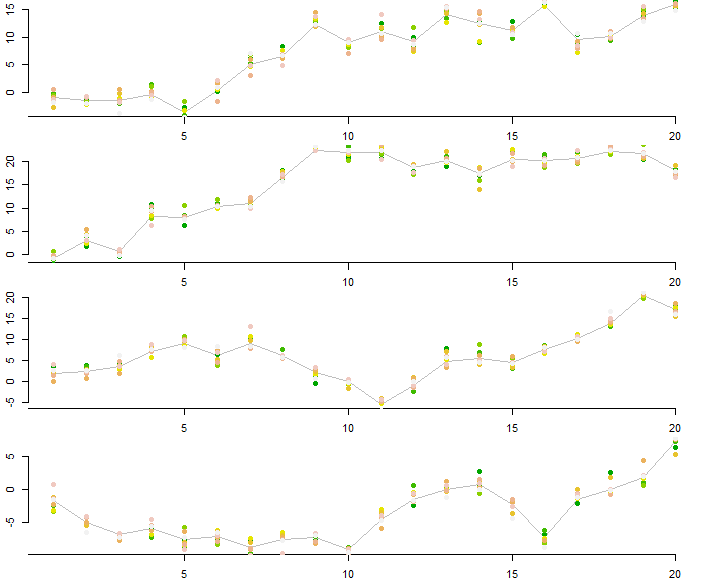
To illustrate, here is an R simulation where all the $\gamma_{t,i}$ are iid.

sim <- function(n.steps=20, n=1, mu=1, sigma=1) {
  gamma <- array(rnorm(n.steps * n, mu, sigma), dim=c(n.steps, n))
  epsilon <- rowSums(gamma)
  x <- cumsum(epsilon)
  y <- x + gamma
  list(x=x, y=y)
}

iter <- function(a) {
  n.steps <- dim(a$y)[1]; n <-dim(a$y)[2] 
  plot(a$x, type="l", col="Gray", frame.plot=FALSE, xaxp=c(0,n.steps,ceiling(n.steps/5)))
  col <- palette(terrain.colors(n))
  i <- 0
  tmp <- apply(a$y, 2, function(z) {i <<- i+1; points(z, pch=19, col=col[i])})
}

set.seed(17)
par(mfrow=c(4,1), mai=c(0.4,0.4,0.0,0.1))
tmp <- replicate(4, iter(sim(20, n=9, mu=0.1)))

Here are four independent realizations of the process:

The step $t$ is on the $x$-axis and the $y$-axis denotes values in the array. The values of $x$ are joined and the corresponding values of $y$ are shown scattered around these values, with colors distinguishing the array components. This array has $9$ values, the drift is $0.1$ per step, and the common variance of the $\gamma_{t,i}$ is $1$.