Appropriate statistical test

Question

I have two sets of data, each having sets of unsigned integers in [0,1,2]. Floating point numbers are not possible.

I have thought to use Welch's t-test, but I don't think that this data is normally distributed, as it's only [0,1,2].

I have heard of parametric tests, and thought of binomial tests (obviously binomial is wrong since I can have 2) but these tests don't seem correct.

Internet searches have only confused me more.

What can of statistical significance test can deal with groups of unsigned integers like this?

Answer 1

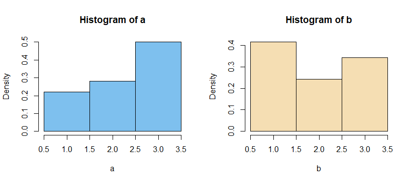
(1) Maybe the issue is whether categories 1,2,3 occur in different proportions in the two samples. This is somewhat like the difference between two binomial proportions, but for three categories instead of two.

set.seed(2020)
a = sample(1:3, 100, rep=T, p=c(1,1,2)/4)
b = sample(1:3,  70, rep=T, p=c(2,1,1)/4)
A=tabulate(a);  B = tabulate(b)
TBL = rbind(A,B); TBL
  [,1] [,2] [,3]
A   22   28   50
B   29   17   24
chisq.test(TBL)

        Pearson's Chi-squared test

data:  TBL
X-squared = 7.7315, df = 2, p-value = 0.02095

A standard chi-squared test for homogeneity of the two samples finds a significant difference at the 3% level.

(2) Maybe 1, 2, 3 are numerical or ordinal and you want to see if one distribution 'dominates' the other.

summary(a);  length(a);  sd(a)
   Min. 1st Qu.  Median    Mean 3rd Qu.    Max. 
   1.00    2.00    2.50    2.28    3.00    3.00 
[1] 100           # sample size
[1] 0.8050347     # sample SD
summary(b);  length(b);  sd(b)
   Min. 1st Qu.  Median    Mean 3rd Qu.    Max. 
  1.000   1.000   2.000   1.929   3.000   3.000 
[1] 70
[1] 0.8734643

[Note: Sample mean and SD are appropriate for numerical data, not for ordinal categorical data.]

par(mfrow=c(1,2))
cutp = .5:3.5
 hist(a, prob=T, br=cutp, col="skyblue2")
 hist(b, prob=T, br=cutp, col="wheat")
par(mfrow=c(1,1))

wilcox.test(a,b)

        Wilcoxon rank sum test with continuity correction

data:  a and b
W = 4269, p-value = 0.009168
alternative hypothesis: true location shift is not equal to 0

The test finds a significant difference between the samples at the 1% level.

Because the two samples are not of the same shape (skewed in opposite directions), it may not be not appropriate to say that significantly different medians indicate a simple shift of the location of a population.

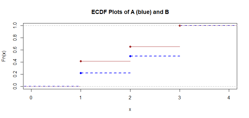
However, empirical CDF (ECDF) plots show that A the dominates B. The ECDF of A (blue) is to the right and below the ECDF of B (brown), where there is a difference. [Perhaps more simply in this example: A has proportionately more 3s and and B has proportionately more 1s.]

plot(ecdf(a), col="blue", lty="dashed", lwd=2, 
     main="ECDF Plots of A (blue) and B")
 lines(ecdf(b), col="brown")

If neither of these scenarios is what you had in mind, maybe you can edit your question to say explicitly why not.