How are missing values exactly handled in C4.5 decision trees?

Question

I quote Tom M. Mitchell's words on this topic:

" A second, more complex procedure is to assign a probability to each of the possible values of A rather than simply assigning the most common value to A(x). These probabilities can be estimated again based on the observed frequencies of the various values for A among the examples at node n. For example, given a boolean attribute A, if node n contains six known examples with A = 1 and four with A = 0, then we would say the probability that A(x) = 1 is 0.6, and the probability that A(x) = 0 is 0.4. A fractional 0.6 of instance x is now distributed down the branch for A = 1, and a fractional 0.4 of x down the other tree branch. These fractional examples are used for the purpose of computing information gain and be further subdivided at subsequent branches of the tree if a second missing value must be tested. This same fractioning of examples can also be applied after learning, to classify new instances whose attribute values are unknown. In this case, the classification of the new instance is simply the most probable classification, computed by summing the weights of the instance fragments classified in different ways at the leaf nodes of the tree. This method for handling missing attribute values is used in C4.5 (Quinlan 1993). "

Now, my questions are:

1. How these fractional 0.6 and 0.4 used to calculate information gain at nodes further down the tree?
2. How would the subdivision take place if a second missing value occurs?
3. How this fractioning would be exactly used in classifying the new examples?

Answer 1

1. I can't find a reference, but the only sensible thing to me is that it operates the same way any sample weighting would: in the information entropy definition $ -\sum_i p_i \log(p_i) $, where normally $p_i=|C_i|/|C|$, we take the total weights instead of just cardinalities.

2. The only sensible thing again: the weights are multiplicative. If a node has 0.4 of a row, and that row needs to be subdivided again in a 0.7 vs 0.3 split, then the children have that row with weights 0.28 and 0.12.

3. This one seems pretty clear from your quote. If the row ends up in four leaves with weights 0.1, 0.2, 0.3, and 0.4, and those leaves get classified as class 1, 2, 3, 1 respectively, then the row gets a total weight for class 1 of 0.1+0.4, weight for class 2 of 0.2, and weight for class 3 of 0.3, and the final classification is class 1. (There's another reasonable approach, I think, if you take the tree to be a soft classifier in the first place. In that case, you'd take the weighted averages of the leaf probabilities.)

---

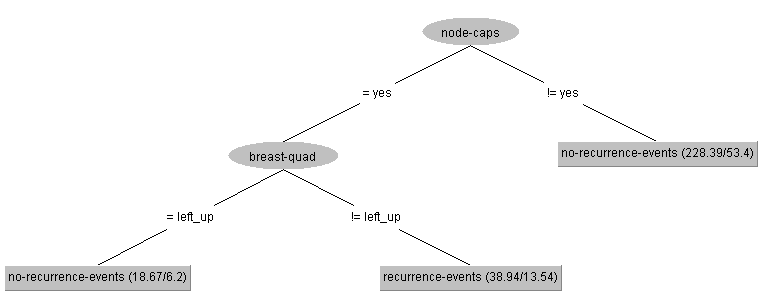
I ran an example through weka's implementation of C4.5. I don't think it preserves the information gain calculations, so I can't confirm (1), but (2) and (3) both check out. I'm using the builtin breast cancer dataset, with just the two features node-caps and breast-quad (the only two with any missing values). I turned off pruning, but enforced only binary splits and set minimum leaf node samples to 10 to keep the tree small. To check (2), I've also taken one row with node-caps=missing, breast-quad=right_low, and class=1 and deleted its breast_quad feature; this is now the sole row missing both features. I set the model to evaluate on the training set.

The first split is on node-caps: there are 222 rows with this feature =no, 56 =yes, and 8=missing. The weights then are $56/278\approx 0.201$ and $0.799$.
node-caps=no reports class 0, 228.39 / 53.4. That $228.39 \approx 222 + 8*0.799$.
As for the $53.4$, we need to check how many no and how many missing are of class 1. That's 51 and 3, respectively, and indeed $53.4 \approx 51 + 3*0.799$.

Using similar calculations for the rest of the tree will allow us to check (2). The node node-caps=yes doesn't give a report since it was split, but we can calculate that it would display $286-228.39=57.61$ and $85-53.4=31.6$. It'll be worth it later to check that the 57.61 is made up of 18 full samples with breast-quad=left_up, 38 full samples with breast-quad!=left_up, and 8 samples with weight 0.201 (of which 3 have left_up, 4 not left_up, and 1 missing).
Now for the second split in this branch; I'll focus on the right one since it is reporting the positive class:
breast-quad!=left_up reports class 1, 38.94 / 13.54. There are 38 rows without missings in this branch, 4 with node-caps missing but breast-quad!=left_up, and 1 with both features missing. So the total weight of samples not missing breast-quad is 38.804; similarly, in the left side of the split, the weight is 18.603. The one row missing both features should now have weight $0.201 * 38.804 / (38.804 + 18.603) \approx 0.136$. And indeed $38.94 = 38.804+0.136$.

Whew, that's way harder to type out than I expected.

For (3) we look to the confusion matrix to see that 38 rows were classified as positive class. That's just the 38 rows without any missings in the leaf we just finished discussing. The one row missing both features got weight 0.799 in the first-level leaf, 0.065 in the other class-0 leaf, and 0.136 in the sole class-1 leaf. The rows missing just node-caps also get weight 0.799 in the first-level leaf, and 0.201 in one or the other second-level leaves. But in any case the 0.799 dominates and they get assigned to class 0. Well, that wasn't convincing.

OK, sorry this is hacky, but I don't want to redo the calculations above right now. We'll keep all that, but now switch the single row that has breast-quad missing in the original dataset from node-caps=no to yes. Now the splits chosen are the same, but this row goes down the left branch, and gets its weight split across the two level-two leaves. Still the weight of the right child is higher, and now this row gets classified as class-1 (total from the confusion matrix is 39).