Your four rules are specifically for a paired t test. If you feel comfortable pretending that Likert-7 data are numerical rather than ordinal, then you
should feel comfortable taking differences in Likert-7 Before and After scores as numerical. You must know that this assumption is somewhat controversial. One question to ask yourself before checking this box, is whether you believe a difference between 2 and 3 on the seven point scale is of the same importance as a difference between 6 and 7 (and similar comparisons).
I also would be very reluctant to prune responses that seem to be outliers. Especially reluctant for differences between two Likert-7 scores which can hardly get really far positive or negative. You are wondering if people change, so you shouldn't be alarmed if some change noticeably more than others.
If the number of subjects is small and the sample distribution of differences is very far from normal in shape, it seems especially risky
to pretend that the data are normal. Because a paired t test is just a
one-sample t test on differences, I would judge normality in terms of differences rather then in terms of before and after Likert scores.
In order to give some examples of tests, I will use R to generate $n = 75$ differences d.
set.seed(403)
x1 = sample(1:7, 75, rep=T, p = c(1,1,2, 2,2,3,1))
x2 = sample(1:7, 75, rep=T, p = c(1,2,2, 3,3,1,1))
d = x2 - x1

summary(d)
   Min. 1st Qu.  Median    Mean 3rd Qu.    Max.
-5.0000 -2.0000 -1.0000 -0.6267  1.0000  5.0000

boxplot(d, horizontal=T, col="skyblue2")

I don't happen to have any outliers, but there is moderate right skewness.
Even so, a Shapiro-Wild test (narrowly) fails to reject these differences
as having come from a normal population.
shapiro.test(d)

        Shapiro-Wilk normality test

data:  d
W = 0.96904, p-value = 0.06298
A one-sample t test on the differences strongly rejects the null hypothesis $H_0: \mu_d = 0$ in favor of $H_a: \mu_d \ne 0$ with P-value about $0.02 < 0.05 = 5\%.$
t.test(d)

        One Sample t-test

data:  d
t = -2.3838, df = 74, p-value = 0.0197
alternative hypothesis: true mean is not equal to 0
95 percent confidence interval:
 -1.1504726 -0.1028607
sample estimates:
  mean of x
 -0.6266667
Of course, I have no idea whether your real data are much like my simulated data. So, I will go looking for trouble that is not really evident in my data. If you want to stay more with the spirit of ordinal categorical data and to avoid an assumption that differences are normally distributed, you could use a paired nonparametric Wilcoxon signed rank test, which finds
a significant difference in location (medians) before vs. after the course.
wilcox.test(x1, x2, paired=T)

        Wilcoxon signed rank test with continuity correction

data:  x1 and x2
V = 1394, p-value = 0.01693
alternative hypothesis: true location shift is not equal to 0
Another possibility is to use the paired t statistic as 'metric' in a
nonparametric permutation test. We believe that this 'metric' is a meaningful way to measure differences before vs. after, but we do not
assume data are normal or that the "t statistic" has any relationship
with a Student t distribution.
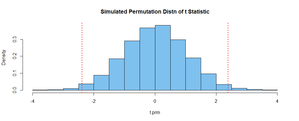
A permutation test: According to the earlier t test, we know that the observed value
t.obs of the t statistic is $-2.3838.$ Then we randomly permute the signs of the differences and find a value t.perm of the sign-permuted data.
By doing this many times we can get an idea of the permutation distribution of the t statistic, and then check to see where t.obs within that distribution.
t.obs = t.test(d)$stat
set.seed(2021)
B = 10000;  t.prm = numeric(B)
for (i in 1:B) {
 d.prm = d * sample(c(-1,1), 75, rep=T)
 t.prm[i] = t.test(d.prm)$stat
}
mean(abs(t.prm) >= abs(t.obs))
[1] 0.024    # P-value of permutation test

hdr = "Simulated Permutation Distn of t Statistic"
hist(t.prm, prob=T, col="skyblue2", main=hdr)
 abline(v = c(t.obs,-t.obs), lwd=2, lty="dotted", col="red")
The (approximate) P-value of the two-tailed permutation test is the
sum of the areas outside the vertical dotted lines in both tails of
the permutation distribution. For my fake dat the P-value is not much
different from the P-value of the paired t test, but for your data
there may be more of a difference.
For the permutation test we are assuming the possibility that subjects
might change up or down on the Likert scale during the course, and that
the data were random samples from the specified testing procedures.
We make no assumption about normality, but the computations to get
the permuted t statistic at each iteration assume that the differences
can be regarded as numeric to the extent that the required means and standard deviations can be
computed. Other metrics involving less arithmetic might be used in
place of the t statistic.

Note: There many possible choices for the 'metric' in a permutation test.
We might have chosen the mean of the differences, with about the same
result. (But for inherently discrete data, such as yours, it would not be a good idea to take the median of the differences because there are too few possible median values to make a useful permutation distribution.)
a.obs = mean(d)
set.seed(1234)
B = 10000;  a.prm = numeric(B)
for (i in 1:B) {
 a.prm[i] = mean(d * sample(c(-1,1), 75, rep=T))
}
mean(abs(a.prm) >= abs(a.obs))
[1] 0.0193  # P-val
length(unique(d))
[1] 11      # highly discrete
length(unique(a.prm))
[1] 83      # enough


