I dput() the data at the bottom in case someone wants to take a look.
ARIMA has a hard time dealing with "long" seasonality, especially if you have only observed two seasonal cycles. "Forecasting with long seasonal periods" by Rob Hyndman is very enlightening reading.
Note that the parameter seasonal=TRUE does not force auto.arima() to use a seasonal model, it only allows it. Use D=1 to force a seasonal model (see Seasonality not taken account of in auto.arima()). Here is what happens then:
> model_sarima <- auto.arima(arrivals,D=1)
> model_sarima
Series: arrivals
ARIMA(2,1,1)(0,1,0)[180]

Coefficients:
         ar1      ar2      ma1
      0.0627  -0.2052  -0.7837
s.e.  0.0895   0.0827   0.0615

sigma^2 estimated as 116.5:  log likelihood=-686.48
AIC=1380.96   AICc=1381.19   BIC=1393.73
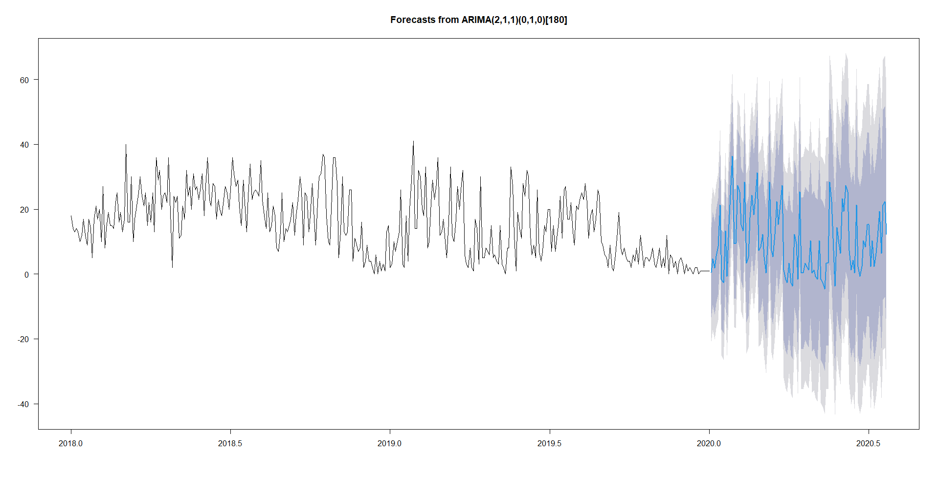
> plot(forecast(model_sarima,h=100),las=1)
As you see, we now have a quite different (and seasonal) model.

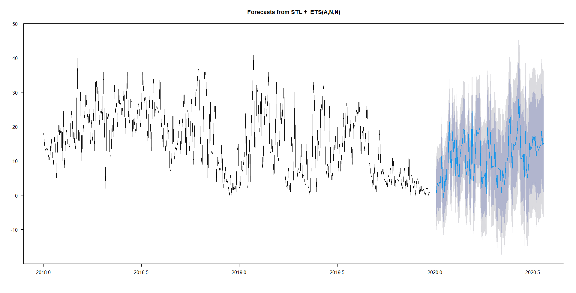
Now the forecasts definitely look more, ahem, sophisticated. Whether they are more accurate is doubtful. For one, some of the point forecasts are negative, which you presumably do not want. Actually, the vast prediction intervals give a hint that auto.arima() does not think this forecast is very useful.
Here is an equally dubious stlf forecast:
plot(stlf(arrivals,h=100),las=1)

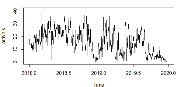
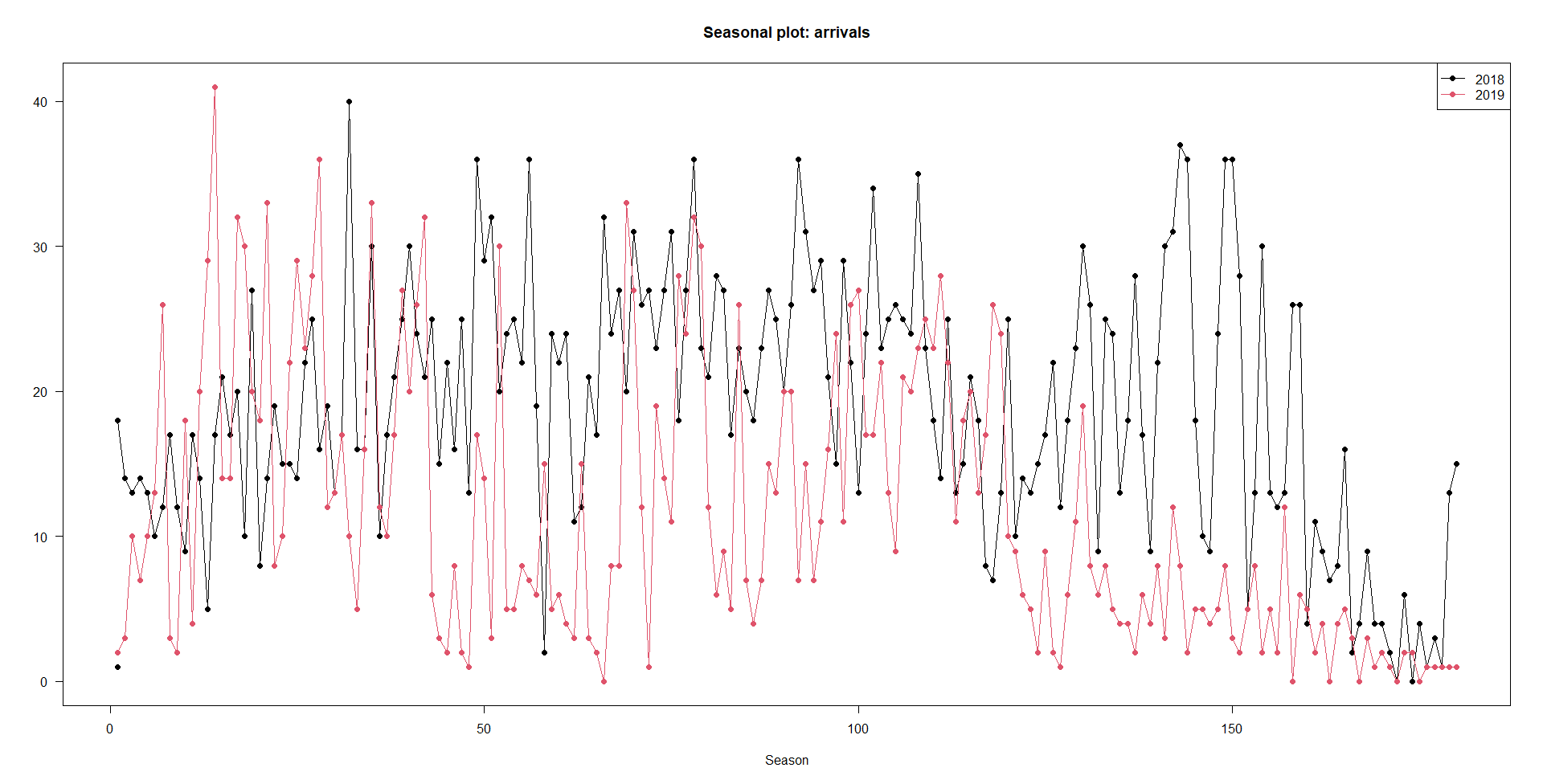
An alternative would be to fit a smooth bump function to your two years of history, then extrapolate this forward. But whatever you do, before you forecast you should really think about that conspicuous drop at the end of your series, which is also visible in a seasonplot. Is this some fundamental change, and will your time series go back to normal, or not, and when? That kind of thinking about the drivers of your series can be far more useful than tweaking ARIMA models.
seasonplot(arrivals,col=1:2,pch=19,las=1)
legend("topright",lwd=1,pch=19,col=1:2,legend=2018:2019)

Data:
arrivals <- structure(c(18L, 14L, 13L, 14L, 13L, 10L, 12L, 17L, 12L, 9L,
17L, 14L, 5L, 17L, 21L, 17L, 20L, 10L, 27L, 8L, 14L, 19L, 15L,
15L, 14L, 22L, 25L, 16L, 19L, 13L, 17L, 40L, 16L, 16L, 30L, 10L,
17L, 21L, 25L, 30L, 24L, 21L, 25L, 15L, 22L, 16L, 25L, 13L, 36L,
29L, 32L, 20L, 24L, 25L, 22L, 36L, 19L, 2L, 24L, 22L, 24L, 11L,
12L, 21L, 17L, 32L, 24L, 27L, 20L, 31L, 26L, 27L, 23L, 27L, 31L,
18L, 27L, 36L, 23L, 21L, 28L, 27L, 17L, 23L, 20L, 18L, 23L, 27L,
25L, 20L, 26L, 36L, 31L, 27L, 29L, 21L, 15L, 29L, 22L, 13L, 24L,
34L, 23L, 25L, 26L, 25L, 24L, 35L, 23L, 18L, 14L, 25L, 13L, 15L,
21L, 18L, 8L, 7L, 13L, 25L, 10L, 14L, 13L, 15L, 17L, 22L, 12L,
18L, 23L, 30L, 26L, 9L, 25L, 24L, 13L, 18L, 28L, 17L, 9L, 22L,
30L, 31L, 37L, 36L, 18L, 10L, 9L, 24L, 36L, 36L, 28L, 5L, 13L,
30L, 13L, 12L, 13L, 26L, 26L, 4L, 11L, 9L, 7L, 8L, 16L, 2L, 4L,
9L, 4L, 4L, 2L, 0L, 6L, 0L, 4L, 1L, 3L, 1L, 13L, 15L, 2L, 3L,
10L, 7L, 10L, 13L, 26L, 3L, 2L, 18L, 4L, 20L, 29L, 41L, 14L,
14L, 32L, 30L, 20L, 18L, 33L, 8L, 10L, 22L, 29L, 23L, 28L, 36L,
12L, 13L, 17L, 10L, 5L, 16L, 33L, 12L, 10L, 17L, 27L, 20L, 26L,
32L, 6L, 3L, 2L, 8L, 2L, 1L, 17L, 14L, 3L, 30L, 5L, 5L, 8L, 7L,
6L, 15L, 5L, 6L, 4L, 3L, 15L, 3L, 2L, 0L, 8L, 8L, 33L, 27L, 12L,
1L, 19L, 14L, 11L, 28L, 24L, 32L, 30L, 12L, 6L, 9L, 5L, 26L,
7L, 4L, 7L, 15L, 13L, 20L, 20L, 7L, 15L, 7L, 11L, 16L, 24L, 11L,
26L, 27L, 17L, 17L, 22L, 13L, 9L, 21L, 20L, 23L, 25L, 23L, 28L,
22L, 11L, 18L, 20L, 13L, 17L, 26L, 24L, 10L, 9L, 6L, 5L, 2L,
9L, 2L, 1L, 6L, 11L, 19L, 8L, 6L, 8L, 5L, 4L, 4L, 2L, 6L, 4L,
8L, 3L, 12L, 8L, 2L, 5L, 5L, 4L, 5L, 8L, 3L, 2L, 5L, 8L, 2L,
5L, 2L, 12L, 0L, 6L, 5L, 2L, 4L, 0L, 4L, 5L, 3L, 0L, 3L, 1L,
2L, 1L, 0L, 2L, 2L, 0L, 1L, 1L, 1L, 1L, 1L, 1L), .Tsp = c(2018,
2020, 180), class = "ts")
