Fitting a curve with data that is nonlinear in logs

Question

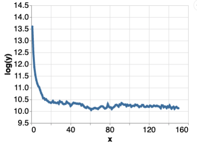
I would like to fit a curve for extrapolation purposes that looks as follows:

The dependent variable is already in logs and the independent variable can be thought of as "days" (i.e. it takes on values 0, 1, 2, 3, 4...). I tried to fit an exponential and a power law model to this data, but the fit was not really good.

I think this is because the data is not linear in logs (at least for the exponential model I am thinking this). Is this correct?

How would you approach such a problem? Are there other types of models that are suitable for data that is non-linear even after taking logs?

Edit: in terms of software, I tried the Exponential and Power law models from the lmfit package (see here, this is a Python package).

Thanks

Answer 1

Seeing that it is a curve fitting regression with just an independent variable that it is easy to visualize, a classic way to deal with non-linearities in the relations is to add new features non-linear in $x$ and then perform a standard linear regression (sometimes this is called linear regression with basis functions).

In this specific case using the lmfit package for me I would use the reciprocal of $x$, i.e $\frac{1}{x}$ and maybe some powers of it too, i.e $\frac{1}{x^2}, \frac{1}{x^2}$ and so on and just use the Model with multiple variables.

Code example, assuming you have an array with $log(y)$ values, let's say ylogged_values and the array of $x$ values called x_values:

from lmfit import Model

def multi_reciprocal_function(x,a0=1, a1=1,a2=1,a3=1):
    return a0 + a1/x + a2/(x**2)+a3*/(x**3)

model = Model(multi_reciprocal_function,independent_vars=['x'])

fit = model.fit(ylogged_values, x = x_values)     

Answer 2

I think you may try a multiple exponential decay, i.e. summing 2 or 3 exponential decays. This because your data after x=25 looks quite linear (considering the dip at 60 as "noise"). But, before launching the fit, play a bit manually with your model function to make sure the automatic optimization starts from reasonable values. The first component should describe the fast decay at the beginning. The second the slow decay at the end. After this you will see if you need another one for the intermediate region. However be careful with extrapolation.. it's always risky if you're not sure the process is still the same after longer times.