23
$\begingroup$

Let say I have following numbers:

4,3,5,6,5,3,4,2,5,4,3,6,5

I sample some of them, say, 5 of them, and calculate the sum of 5 samples. Then I repeat that over and over to get many sums, and I plot the values of sums in a histogram, which will be Gaussian due to the Central Limit Theorem.

But when they are following numbers, I just replaced 4 with some big number:

4,3,5,6,5,3,10000000,2,5,4,3,6,5

Sampling sums of 5 samples from these never becomes Gaussian in histogram, but more like a split and becomes two Gaussians. Why is that?

$\endgroup$
6
  • 1
    $\begingroup$ It won’t do that if you increase it to beyond n = 30 or so ... just my suspicion and more succinct version / restating of the accepted answer below. $\endgroup$
    – oemb1905
    Commented Mar 10, 2019 at 0:50
  • $\begingroup$ @JimSD the CLT is an asymptotic result (i.e. about the distribution of standardized sample means or sums in the limit as sample size goes to infinity). $n=5$ is not $n\to\infty$. The thing you're looking at (the approach toward normality in finite samples) is not strictly a result of the CLT, but a related result. $\endgroup$
    – Glen_b
    Commented Mar 10, 2019 at 11:30
  • 3
    $\begingroup$ @oemb1905 n=30 is not sufficient for the sort of skewness OP is suggesting. Depending on how rare that contamination with a value like $10^7$ is it might take n=60 or n=100 or even more before the normal looks like a reasonable approximation. If the contamination is about 7% (as in the question) n=120 is still somewhat skew $\endgroup$
    – Glen_b
    Commented Mar 10, 2019 at 11:42
  • 2
    $\begingroup$ Possible duplicate of Why does increasing the sample size of coin flips not improve the normal curve approximation? $\endgroup$ Commented Mar 10, 2019 at 21:32
  • $\begingroup$ Think that values in intervals like (1,100,000 , 1,900,000) will never be reached. But if you make means of a decent amount those sums, it will work! $\endgroup$
    – David
    Commented Mar 11, 2019 at 7:42

4 Answers 4

20
$\begingroup$

Let's recall, precisely, what the central limit theorem says.

If $X_1, X_2, \cdots, X_k$ are independent and identically distributed random variables with (shared) mean $\mu$ and standard deviation $\sigma$, then $\frac{X_1 + X_2 + \cdots + X_k}{k\frac{\sigma}{\sqrt{k}}}$ converges in distribution to a standard normal distribution $N(0, 1)$ (*).

This is often used in the "informal" form:

If $X_1, X_2, \cdots, X_k$ are independent and identically distributed random variables with (shared) mean $\mu$ and standard deviation $\sigma$, then $X_1 + X_2 + \cdots + X_k$ converges "in distribution" to a standard normal distribution $N(k \mu, \sqrt{k} \sigma)$.

There's no good way to make that form of the CLT mathematically precise, since the "limit" distribution change, but it's useful in practices.

When we have a static list of numbers like

4,3,5,6,5,3,10000000,2,5,4,3,6,5

and we are sampling by taking a number at random from this list, to apply the central limit theorem we need to be sure that our sampling scheme satisfies these two conditions of independence and identically distributed.

  • Identically distributed is no problem: each number in the list is equally likely to be chosen.
  • Independent is more subtle, and depends on our sampling scheme. If we are sampling without replacement, then we violate independence. It is only when we sample with replacement that the central limit theorem is applicable.

So, if we use with replacement sampling in your scheme, then we should be able to apply the central limit theorem. At the same time, you are right, if our sample is of size 5, then we are going to see very different behaviour depending on if the very large number is chosen, or not chosen in our sample.

So what's the rub? Well, the rate of convergence to a normal distribution is very dependent on the shape of the population we are sampling from, in particular, if our population is very skew, we expect it to take a long time to converge to the normal. This is the case in our example, so we should not expect that a sample of size 5 is sufficient to show the normal structure.

Three Normal Distributions

Above I repeated your experiment (with replacement sampling) for samples of size 5, 100, and 1000. You can see that the normal structure is emergent for very large samples.

(*) Note there are some technical conditions needed here, like finite mean and variance. They are easily verified to be true in our sampling from a list example.

$\endgroup$
6
  • $\begingroup$ Thank you for a very quick and perfect answer. Idea of CLT, replacement, the need for more samples when data distribution is skewed,... It is very clear now. My original intention of question is, just as you mentioned, the case when one large number is included without replacement and the number of sampling is fixed. It behaves very differently, and therefore we need to consider "conditional" CLT for the case a large number is sampled and the case not sampled. I wonder if there is any research or prior work for that.. But thank you anyway. $\endgroup$
    – JimSD
    Commented Mar 9, 2019 at 7:09
  • $\begingroup$ don't know if applicable here, but theorem of CLT convergence regulated by skewness en.wikipedia.org/wiki/Berry%E2%80%93Esseen_theorem $\endgroup$
    – seanv507
    Commented Mar 9, 2019 at 15:56
  • $\begingroup$ I'm a bit confused by @MatthewDrury's definition of the CLT. I think that $\frac{\sum X_k}{k}$ converges to a constant by the LLN, not a normal distribution. $\endgroup$
    – JTH
    Commented Mar 9, 2019 at 17:41
  • 1
    $\begingroup$ @seanv507 absolute third moment, rather than skewness; the two are related but note that for a symmetric distribution with finite third moment that the Berry-Esseen bound on $|F_n(x)-\Phi(x)|$ is not 0 because $\rho/\sigma^3$ is not skewness $\endgroup$
    – Glen_b
    Commented Mar 10, 2019 at 11:28
  • 1
    $\begingroup$ @Glen_b Yah, I was being a bit informal (which I perhaps should not have been), but I can fix that up this afternoon since it's led to a bit of confusion. $\endgroup$ Commented Mar 10, 2019 at 16:46
13
$\begingroup$

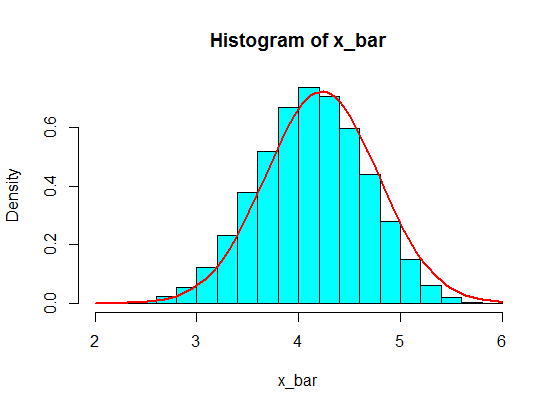
In general, the size of each sample should be more than $5$ for the CLT approximation to be good. A rule of thumb is a sample of size $30$ or more. But, with the population of your first example, $5$ is OK.

pop <- c(4, 3, 5, 6, 5, 3, 4, 2, 5, 4, 3, 6, 5)
N <- 10^5
n <- 5
x <- matrix(sample(pop, size = N*n, replace = TRUE), nrow = N)
x_bar <- rowMeans(x)
hist(x_bar, freq = FALSE, col = "cyan")
f <- function(t) dnorm(t, mean = mean(pop), sd = sd(pop)/sqrt(n))
curve(f, add = TRUE, lwd = 2, col = "red")
enter image description here

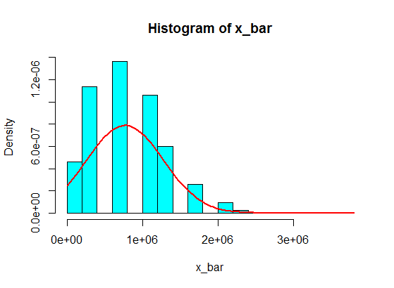
In your second example, because of the shape of the population distribution (for one thing, it's too much skewed; read the comments by guy and Glen_b bellow), even samples of size $30$ won't give you a good approximation for the distribution of the sample mean using the CLT.

pop <- c(4, 3, 5, 6, 5, 3, 10000000, 2, 5, 4, 3, 6, 5)
N <- 10^5
n <- 30
x <- matrix(sample(pop, size = N*n, replace = TRUE), nrow = N)
x_bar <- rowMeans(x)
hist(x_bar, freq = FALSE, col = "cyan")
f <- function(t) dnorm(t, mean = mean(pop), sd = sd(pop)/sqrt(n))
curve(f, add = TRUE, lwd = 2, col = "red")
enter image description here

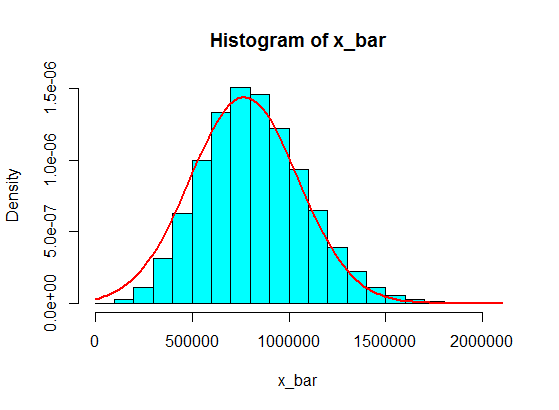
But, with this second population, samples of, say, size $100$ are fine.

pop <- c(4, 3, 5, 6, 5, 3, 10000000, 2, 5, 4, 3, 6, 5)
N <- 10^5
n <- 100
x <- matrix(sample(pop, size = N*n, replace = TRUE), nrow = N)
x_bar <- rowMeans(x)
hist(x_bar, freq = FALSE, col = "cyan")
f <- function(t) dnorm(t, mean = mean(pop), sd = sd(pop)/sqrt(n))
curve(f, add = TRUE, lwd = 2, col = "red")
enter image description here

$\endgroup$
6
  • 3
    $\begingroup$ It’s not the variance that is problem. One way of getting rigorous control is using the ratio of the third central moment to the standard deviation cubed, as in the Berry-Esseen theorem. $\endgroup$
    – guy
    Commented Mar 9, 2019 at 4:02
  • $\begingroup$ Perfect. Added. Tks. $\endgroup$
    – Zen
    Commented Mar 9, 2019 at 4:06
  • 1
    $\begingroup$ Thank you for a quick, visual, and perfect answer with a code. I was very surprised how quick it was! I was not aware of the appropriate number of sampling. I was thinking of the case where the number of sampling is fixed. $\endgroup$
    – JimSD
    Commented Mar 9, 2019 at 7:05
  • $\begingroup$ @guy, Thank you for the that. I didn't know the idea of "the ratio of the third central moment to the standard deviation cubed in Berry-Esseen theorem". I just wish to tackle the case where there is one large number like outlier is included in distribution. And that kind of distribution can be refereed to as you mentioned, I suppose. If if you know any prior work dealing with that kind of distribution, let me know, thank you. $\endgroup$
    – JimSD
    Commented Mar 9, 2019 at 7:25
  • 2
    $\begingroup$ @guy the Berry Esseen theorem is about third absolute moment about the mean $\rho=E[|X-\mu|^3]$ not just the third moment about the mean $\mu_3=E[(X-\mu)^3]$. This makes it responsive to not just skewness but also heavy tails. $\endgroup$
    – Glen_b
    Commented Mar 10, 2019 at 11:47
7
$\begingroup$

I'd just like to explain, using complex cumulant-generating functions, why everyone keeps blaming this on skew.

Let's write the random variable you're sampling as $\mu+\sigma Z$, where $\mu$ is the mean and $\sigma$ the standard deviation so $Z$ has mean $0$ and variance $1$. The cumulant-generating function of $Z$ is $-\frac{1}{2}t^2-\frac{i\gamma_1}{6}t^3+o(t^3)$. Here $\gamma_1$ denotes the skew of $Z$; we could write it in terms of the skew $\kappa_3$ of the original variable $\mu+\sigma Z$, viz. $\gamma_1=\sigma^{-3}\kappa_3$.

If we divide the sum of $n$ samples of $Z$'s distribution by $\sqrt{n}$, the result has cgf $$n\left(-\frac{1}{2}\left(\frac{t}{\sqrt{n}}\right)^2-\frac{i\gamma_1}{6}\left(\frac{t}{\sqrt{n}}\right)^3\right)+o(t^3)=-\frac{1}{2}t^2-\frac{i\gamma_1}{6\sqrt{n}}t^3+o(t^3).$$For a Normal approximation to be valid at large enough $t$ for the graph to look right, we need sufficiently large $n$. This calculation motivates $n\propto\gamma_1^2$. The two samples you considered have very different values of $\gamma_1$.

$\endgroup$
-1
$\begingroup$

Short answer is, you don't have a big enough sample to make central limit theorem apply.

$\endgroup$
4
  • 1
    $\begingroup$ That this cannot be a valid explanation is evident from the observation that the CLT gives a good approximation for the first set of data in the question, which is equally small. $\endgroup$
    – whuber
    Commented Mar 9, 2019 at 15:45
  • $\begingroup$ @whuber: I think you are saying that the normal distribution gives a reasonably good approximation for a sample of five from the first set. Since there are only an finite number of values for the sums (13 possible values without replacement and 21 possible values with replacement), the approximation does not get much better with a large number of samples of five, and the initial approximation is more due to the initial pattern... $\endgroup$
    – Henry
    Commented Mar 9, 2019 at 16:49
  • $\begingroup$ @whuber Since the distribution of the first set looks left skewed, I would expect the sum of five also to be left skewed, in a less extreme way than I would expect the sum of five from the second set to be right skewed. To get the skewness to reduce further, I would have thought that you would need a larger sample size $\endgroup$
    – Henry
    Commented Mar 9, 2019 at 16:51
  • 1
    $\begingroup$ @Henry Thank you for your comments. I wasn't making a remark about these particular circumstances, but only about the logic of this answer, in the hope that it could be explained further. $\endgroup$
    – whuber
    Commented Mar 9, 2019 at 18:33

Your Answer

By clicking “Post Your Answer”, you agree to our terms of service and acknowledge you have read our privacy policy.

Not the answer you're looking for? Browse other questions tagged or ask your own question.