Best way to compare two treatment groups to a control

Question

I'm trying to compare two different fertilizer treatments to a control group (no fertilizer). I ran a model like this:

plants_lm <- lm(weight ~ group, data = plants)

summary(plants_lm)

Call:
lm(formula = weight ~ group, data = plants)

Residuals:
    Min      1Q  Median      3Q     Max 
-1.0710 -0.4180 -0.0060  0.2627  1.3690 

Coefficients:
                 Estimate Std. Error t value Pr(>|t|)    
(Intercept)        5.0320     0.1971  25.527   <2e-16 ***
groupFertlizer_A  -0.3710     0.2788  -1.331   0.1944    
groupFertlizer_B   0.4940     0.2788   1.772   0.0877 .  
---
Signif. codes:  0 ‘***’ 0.001 ‘**’ 0.01 ‘*’ 0.05 ‘.’ 0.1 ‘ ’ 1

Residual standard error: 0.6234 on 27 degrees of freedom
Multiple R-squared:  0.2641,    Adjusted R-squared:  0.2096 
F-statistic: 4.846 on 2 and 27 DF,  p-value: 0.01591

I'm a little confused as to how to interpret these results. The only significant result is the control. What does this mean exactly? I feel like I'm doing something wrong, because what I want to know is whether the other two groups are different from the control. Hope this makes some sense.

Answer 1

Your variable group is a factor with three levels, control, Fertilizer_A, Fertilizer_B, and control is used as reference )or baseline) level, so its implied coefficient is zero. See What to do in a multinomial logistic regression when all levels of DV are of interest?.

The coefficients for the two non-reference levels, Fertilizer_A and Fertilizer_B represent in fact contrast comparing those levels to the control. You say:

The only significant result is the control.

and I do not understand what you come to that conclusion. The last line in your output

F-statistic: 4.846 on 2 and 27 DF,  p-value: 0.01591

represent a comparison between your model and the intercept-only model, which is the null hypothesis model representing the null that the fertilizer treatment has no effect. That hypothesis test has the p-value 0.01591, which is often considered significant, for instance, at the conventional 5% level you can reject the null that the fertilizer treatment has no effect.

Edit

The two individual p-values in the output table each test two separate contrasts, comparing A with control and comparing B with control. That neither of those are significant at the conventional 5% level, while the overall test is significant, only says that we have some information to say that fertilizer use is different from control, but not sufficient information to say which fertilizer is different from control. This might be seen as a paradox, but is not: An equivalent example is that police might be able to prove that either A or B murdered the victim, but not enough to say which of them.

In this case, from the point estimates, A seems worse than control while B seems better. Detailed interpretation will depend on knowledge of the fertilizers used etc, but might also indicate need of further replicate experiments to give a better conclusion. Note that the conclusion from the overall test (which is two-sided) only is that fertilizer id different from control, not better than.

As for comparing the two treatments, that is also a contrast, and all contrasts can be tested. In the following I will abbreviate the levels with A, B, C. The two printed contrasts are A-C and B-C, note that we can write A-B as A-C - (B-C), so from the output you can find the point estimate as A-C = -0.3710 - 0.4940, but to calculate the t-test you also need then standard error, which you need further information from. But you can calculate it yourself using the covariance matrix of the coefficient vector, which you get by the call vcov(plants_lm), or you can use use a function like car::linearHypothesis to do it. For another way see the code at Categorical variable coding to compare all levels to all levels

Answer 2

kjetil's answer explains well the interpretation of the two coefficients from your model as contrasts between each fertilizer and control.

You can use the package contrast to explicitly perform the final contrast, between the two fertilizers. First, simulating data and fitting a model as you did:

library("contrast")
library("ggplot2")
set.seed(42)

## simulate a plants df with minor differences between each group
plants <- data.frame(
    weight = c(rnorm(50), rnorm(50, mean = 0.2), rnorm(50, mean = 0.3)),
    group = factor(rep(c("control", "treat1", "treat2"), each = 50))
)

fit <- lm(
    weight ~ group,
    data = plants
)
summary(fit)
#> 
#> Call:
#> lm(formula = weight ~ group, data = plants)
#> 
#> Residuals:
#>      Min       1Q   Median       3Q      Max 
#> -3.09379 -0.57597  0.00902  0.57207  2.85314 
#> 
#> Coefficients:
#>             Estimate Std. Error t value Pr(>|t|)  
#> (Intercept) -0.03567    0.14241  -0.250    0.803  
#> grouptreat1  0.33637    0.20139   1.670    0.097 .
#> grouptreat2  0.18442    0.20139   0.916    0.361  
#> ---
#> Signif. codes:  0 '***' 0.001 '**' 0.01 '*' 0.05 '.' 0.1 ' ' 1
#> 
#> Residual standard error: 1.007 on 147 degrees of freedom
#> Multiple R-squared:  0.01868,    Adjusted R-squared:  0.00533 
#> F-statistic: 1.399 on 2 and 147 DF,  p-value: 0.2501

Now, to perform contrasts. Note, the first two are redundant because they correspond to the latter two rows of the summary table above, but they're shown for clarity.

contrast(fit,
    a = list(group = "treat1"),
    b = list(group = "control")
)
#> lm model parameter contrast
#> 
#>    Contrast      S.E.       Lower     Upper    t  df Pr(>|t|)
#> 1 0.3363732 0.2013913 -0.06162303 0.7343694 1.67 147    0.097
contrast(fit,
    a = list(group = "treat2"),
    b = list(group = "control")
)
#> lm model parameter contrast
#> 
#>    Contrast      S.E.      Lower     Upper    t  df Pr(>|t|)
#> 1 0.1844207 0.2013913 -0.2135755 0.5824169 0.92 147   0.3613
contrast(fit,
    a = list(group = "treat2"),
    b = list(group = "treat1")
)
#> lm model parameter contrast
#> 
#>     Contrast      S.E.      Lower     Upper     t  df Pr(>|t|)
#> 1 -0.1519525 0.2013913 -0.5499487 0.2460437 -0.75 147   0.4517
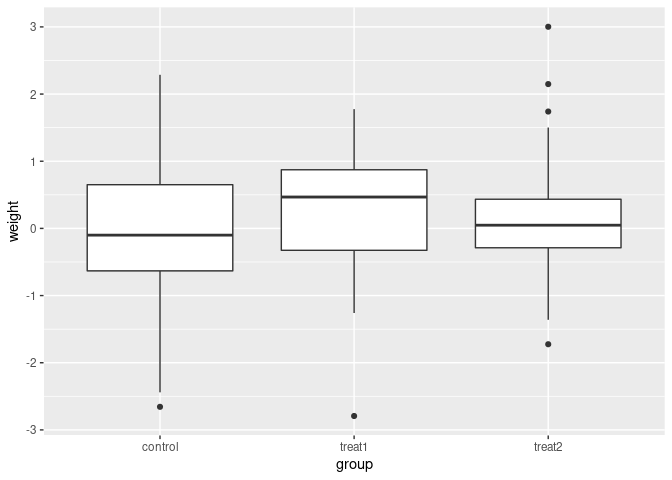
ggplot(plants) +
    aes(group, weight) +
    geom_boxplot()

Disclaimer: I'm the maintainer, though not the developer, of contrast.

Answer 3

This question comes up a lot and there is a method that answers all the questions you have. Look at Ways of comparing linear regression interepts and slopes?. It explains how to compare slopes and intercepts of as many groups as you want and will tell you the difference between groups.