Inconsistent posterior estimates in Beta-Binomial likelihood vs Binomial in Bayesian, multilevel models?

Question

In this Google Colab, I've simulated Binomial count data and compared the performance of Binomial-likelihood and Beta-Binomial-likelihood models. Both models have the same Beta prior on theta, the rate parameter. And in multilevel fashion, its alpha and beta parameters have their own priors (each half-normal.) Likewise, much of these same details are captured in PyMC3 discourse.

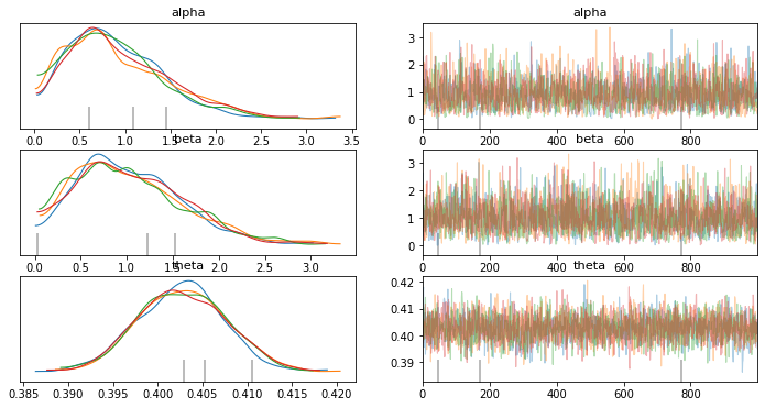
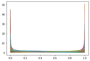
In both cases inference on the mean value of theta was really close to what I specified in simulations. However, I noticed something perplexing. In the binomial model, the inferred posterior distributions were inconsistent. Namely, the expectation of theta given alpha and beta differed from the expectation of theta $E[P(\theta|E[\alpha], E[\beta])] \neq E[P(\theta)]$.

PyMC3 posterior plots:

Posterior Theta given alpha, beta:

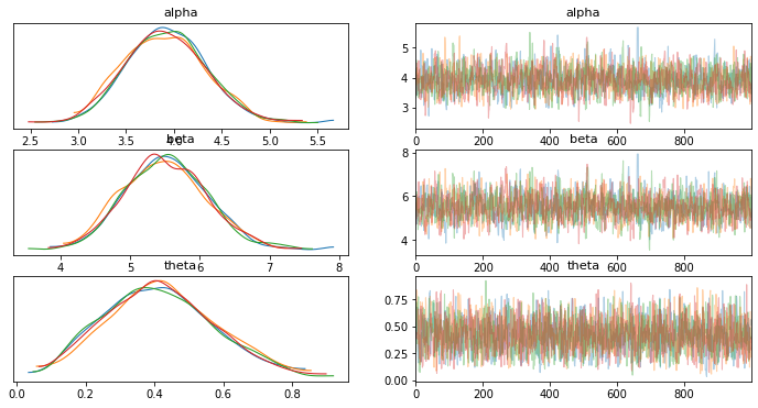
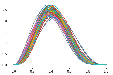
This puzzled me. And so for comparison, I swapped the Binomial-likelihood out for a Beta-Binomial likelihood. The expectation of theta equals the expectation of theta given alpha and beta $E[P(\theta|E[\alpha], E[\beta])] = E[P(\theta)]$.

PyMC3 posterior plots:

Theta given alpha,beta posterior:

On the surface this seems intuitive; alpha and beta were not part of the Binomial likelihood function and so there wasn't any "message passing" from theta to alpha and beta. Hence, their posterior estimates are nonsense.

But the more I thought about this, the more I realized that this brings into question my understanding of multilevel models altogether. I had thought that one could put priors on priors with a multilevel model and infer the distribution of every parameter in the model, not just the parameters explicitly referenced in the likelihood function. Now I'm not so sure...

Perhaps a custom likelihood function is needed for every multilevel model in order to combat nonsense parameter estimates (aka you can't rely on multilevel priors to effectively pass messages between parameters?)

Or perhaps I made some design decisions in my data simulation that are nuanced and not ideal for the Binomial likelihood model?

Edit: It's worth noting how the plots "Posterior of Theta given alpha and Beta" are generated. Some data is captured below, the python function is below:

def sample_post_plot(samples=100, trace_obj=trace1):
  X = np.linspace(0,1,1000)  
  for i in range(samples):
    idx = random.randint(0,len(trace_obj.get_values('alpha')))
    a = trace_obj.get_values('alpha')[idx]
    b = trace_obj.get_values('beta')[idx]
    Y = stats.beta(a=a,b=b).pdf(X)
    plt.plot(X,Y)  

Some notes:

1. trace_obj is an object returned by PyMC3 post-inference.
2. The method get_values('parameter')[idx] returns the specific value that the parameter took on at a specific index in the chain.
3. I uniformly sample an index (location in the chain) and use it to retrieve the specific $\alpha, \beta$ values observed at that index in the chain.
4. I use these $\alpha, \beta$ in conjunction with scipy's stats.beta(a,b).pdf(X) to evaluate the likelihood of each $x_i$ in the range [0,1].
5. I repeat this iteratively according to the argument samples=100. Thus I sample $P(\theta|\alpha,\beta)$.
6. We observe that, for the Binomial likelihood model, this plot is completely different from PyMC3's posterior chain over $\theta$. So it's my conclusion that PyMC3's inferred $\alpha, \beta$ distributions are nonsense.

Answer 1

I posted a similar question at the PyMC3 discourse. The answer was to do proper multilevel modeling/pooling. Essentially, I should have one $\theta$ per observation and each one should be "communicate" with one another through the common $\alpha$ and $\beta$ parameters. The results were identical to having used the Beta-Binomial likelihood.

It seems that trying to infer a single $\theta$, it wasn't able to vary as knowledge of $\alpha, \beta$ determined it, exactly (and conversely.) But by turning $\theta$ into a vector, rather than a scalar, I got good inference on $\alpha, \beta$.

with pm.Model() as m1:
  alpha = pm.HalfNormal('alpha',sigma=1)
  beta = pm.HalfNormal('beta',sigma=1)
  theta = pm.Beta('theta',alpha, beta, shape=len(W))
  lik = pm.Binomial('likelihood',n=N,p=theta,observed=W)
  trace1 = pm.sample(chains=4)