3
$\begingroup$

I have a synthetic measurement model that looks like this,

$$ x(t) = e^{j u t \frac{4}{\lambda}}, $$ $\lambda$ is a constant.

$$ z(t) = x(t) + n(t) $$

The quantity $j = \sqrt{-1}$, the imaginary unit. The noise $n(t)$ added to this signal has two components as well, one real and one imaginary part.

Where $n$ is a zero mean white Gaussian noise with a variance of $\sigma_n^2$. $$ n = \frac{1}{\sqrt{2}} \left( \mathcal{N}(0, \sigma_n^2) + j \mathcal{N}(0, \sigma_n^2) \right) $$

From this measurement model, I take only some measurements for analysis of the MCMC method.

I want to estimate the value of $u$ from this model. The noise $n$ has both a real and an imaginary part. I assume that the noise variance $\sigma_n$ is known already.

I use a Gaussian prior for $u$. The parameter $u$ is not complex; it is a real quantity.

$$ p(u) = \mathcal{N}(\mu_u, \sigma_u) $$

The likelihood I take as,

$$ \log(p(z|u)) = -\frac{1}{2} (\mathbf{z} - \mathbf{x})^T K^{-1} (\mathbf{z} - \mathbf{x}) $$

Where $\mathbf{z}$ and $\mathbf{x}$ are vectors with the dimension of $t$. The value $K$ is defined as,

$$ K = \sigma^2 \times I, $$ $I$ is the identity matrix. So, $K$ is a real matrix dealing only with the known noise variance.

I separately compute the real and imaginary parts of the likelihood as,

$$ \log(p(z_{Real}|u)) = -\frac{1}{2} (real(\mathbf{z}) - real(\mathbf{x}))^T K^{-1} (real(\mathbf{z}) - real(\mathbf{x})) $$

$$ \log(p(z_{Imag}|u)) = -\frac{1}{2} (imag(\mathbf{z}) - imag(\mathbf{x}))^T K^{-1} (imag(\mathbf{z}) - imag(\mathbf{x})) $$

The problem I face is that the likelihood not only has a real, but also has a imaginary component. In the acceptance criteria of Matropolis Haistings algorithm, I now add the real and imaginary likelihoods in log scale. Code is given later in this post.

If the ground truth has $1000$ samples, only $50$ samples are available as measurements. The samples are placed in a way that there is a definite gap between sets of samples. For example, $5$ samples placed together in time $t$, there is a huge time gap of $95$ sample space and again another $5$ samples are available. The samples in time $t$ available can be represented as this.

$$t = N.k.dT + \sum_{i = 1}^{M}i.dT$$

Here, $N = 100$, $M = 5$ and $k \; \epsilon \; [0, 1, 2, ....]$.

A working example is given below.


%% HD signal generator

close all;
clear;

SNR_db = 20;                % Noise is added with a given SNR in dB
SNR = 10^(SNR_db/10);       % SNR in linear scale


lambda = 1;             

r0 = 0;                     
u = 1;                      % Ground truth u

N = 100; 
M = 5;

K = linspace(1, 10, 10);

Nt = K(end) * N;                 % Number of Truth samples (N * M * 20)

dT = 0.1;                  % t step
r(1) = r0;                  

Z(1) = exp(1j * 4 * pi/lambda .* r(1)); 

for i = 2:Nt
    r(i) = r(i - 1) + u * dT;
    Z(i) = exp(1j * 4 * pi/lambda .* r(i)); % Ground truth samples
end

Noise = sum(abs(Z).^2)./(Nt .* SNR);         % Finding Noise power and ...
                                             %noise variance with the data and given SNR
sigma_n = sqrt(Noise);

Z_model = Z + sigma_n .* (randn(1, Nt) + 1j .* randn(1, Nt))./sqrt(2); % Adding complex noise 


%% Available samples [Measurement model with only a few samples]


Z_model_re = reshape(Z, [N K(end)]); 
Z_avail = Z_model_re(1:M, :); 

Z_avail_vec_ = reshape(Z_avail, [M * K(end) 1]); % available samples for measurements


Z_avail_vec = Z_avail_vec_ + sigma_n .* (randn(1, length(Z_avail_vec_)).'+ 1j .* randn(1, length(Z_avail_vec_)).')./sqrt(2);

for k = 1:K(end)
    t(:, k) = (k - 1) * N + [1:M]; % This for loop calculates the t instances of the available samples
end

t_avail = reshape(t, [length(Z_avail_vec) 1]) .* dT; % vectorize the available time instances


%% MCMC parameters in a structure var

% E is the structure having options for MCMC

E.n = 1;                            % Number of variables to be estimated

E.E0 = [1.3];                    % Initial value of u 
E.sig = [50000];                    % Initial value of the Std of the prior of u 


%% This section has MCMC algorithm 
No_iter = 10000; % Number of iterations

[accepted, rejected, itern, E_new] = MHu(E, No_iter, Z_avail_vec, t_avail, r0, sigma_n);

%% Plot MCMC outputs 


for i = 1:E.n

    
   figure(1000+i);plot(rejected(:, i)); hold on; plot(accepted(:, i)); % Accepted and rejected values
   
   burnin = round(0.25 * length(accepted(:, i)));                      % 25% of the data is taken as burnin
   figure(2000+i); histogram(accepted(burnin+1:end, i), 100);          % histogram of accepted
   burninrej = round(0.25 * length(rejected(:, i)));                   % Burnin for rejected
   figure(3000+i); histogram(rejected(burninrej+1:end, i), 100);       % Burnin for accepted
   mu_re = mean(accepted(burnin+1:end, i));                            % Mean of accepted 
   rej_re = mean(rejected(burnin+1:end, i));                           % Mean of rejected
end


function [accepted, rejected, itern, E] = MHu(E, iter, data, t_avail, r0, sigma_n)

%% Inputs:

% E - Struct of MCMC options 
% iter - number of iterations
% data - data available
% t_avail - t instances of the data
% r0 - start position of the target - assumed to be known
% sigma_n - noise standard deviation - assumed to be known

%% Outputs:

% accepted - accpetd values
% rejected - rejected values 
% itern - iterations at which we accept a value
% E - the new Struct of MCMC options after processing - A new E.sig is
% updated


    u = E.E0; % save the initial value in u
    accepted = zeros(1, E.n); 
    rejected = zeros(1, E.n);
    
    
    itern = 0;
    
    for i = 1:iter
        disp(i);
        [u_new, punew, pu] = TMu(u, E.sig);     % u_new is a new sample drawn for u 
                                                % prior probability of u_new
                                                % prior probability of u 
        
        u_lik = LLu(u, data, t_avail, r0, sigma_n, pu); % Likelihood of u wth data
        u_new_lik = LLu(u_new, data, t_avail, r0, sigma_n, punew); % Likelihood of u_new with data
   
%% Acceptance Logic

        if (acceptance((u_lik), (u_new_lik)))
            
            
            accepted = [accepted; u_new];
            itern = [itern i];             
            u = u_new;
        else
            rejected = [rejected; u_new];
        end
    end
end
function [unew, punew, pu] = TMu(u, Esigma)

    for i = 1:length(Esigma)
        unew(i) = normrnd(u(i), Esigma(i), 1); % Draw a new value
        
        
        pu(i) = normpdf(u(i), u(i), Esigma(i)); % Find the prior probability of x
        punew(i) = normpdf(unew(i), u(i), Esigma(i)); % Find the prior probability of y
    end 
end


function ret = LLu(u, data, t_avail, r0, sigma_n, pu)

    lambda = 0.03;
    
    r(1) = r0; % initial position of the scatterer
    Z_model(1) = exp(1j .* 4 .* pi/lambda .* r(1)); % First sample echo model 
    
    for l = 2:length(t_avail)
            r(l) = r(l - 1) + u .* (t_avail(l) - t_avail(l - 1)); 
            % This for loop calculates the model
            % samples from the available t steps $t_avail$
          Z_model(l) = exp(1j .* 4 .* pi/lambda .* r(l));
    end
    
    Nt = length(data);
   
    K = eye(Nt, Nt) .* sigma_n.^2; % Noise diagnoal matrix with size length(t_avail) x length(t_avail)
   

%% Real and imaginary part likelihood 

    ret_re = log(pu) -Nt/2 .* log(2*pi) - 1/2 * (real(data) - real(Z_model).').' * inv(K) * (real(data) - real(Z_model).');
    ret_im = log(pu) -Nt/2 .* log(2*pi) - 1/2 * (imag(data) - imag(Z_model).').' * inv(K) * (imag(data) - imag(Z_model).');
    
    ret = ret_re + ret_im; % Total likelihood (multiplication of real and imaginary likelihoods in linear scale)
    

end

function ret = acceptance(u, u_new)
   
        alpha = exp(u_new - u);
        rnd = rand;
        
    if alpha > rnd
        ret = 1;
    else
        ret = 0;
        %accept = rand;
        %ret = (accept < exp(x_new - x));
%         ret = 0;
    end
end

Total truth samples: 1000 Total measurement samples: 50 True u : 1 (as per the code above)

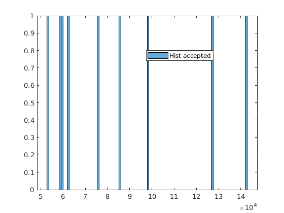
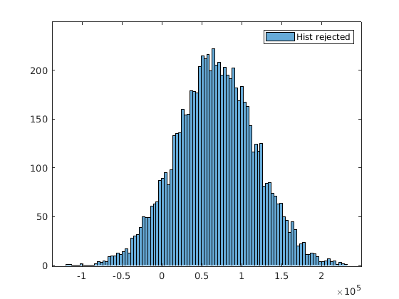
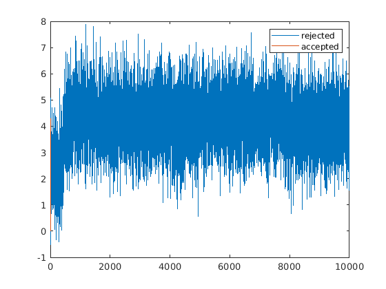
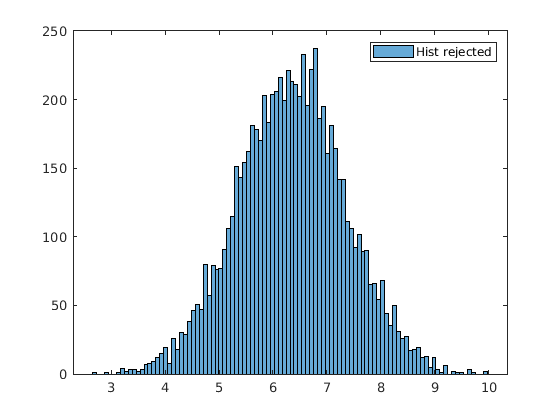
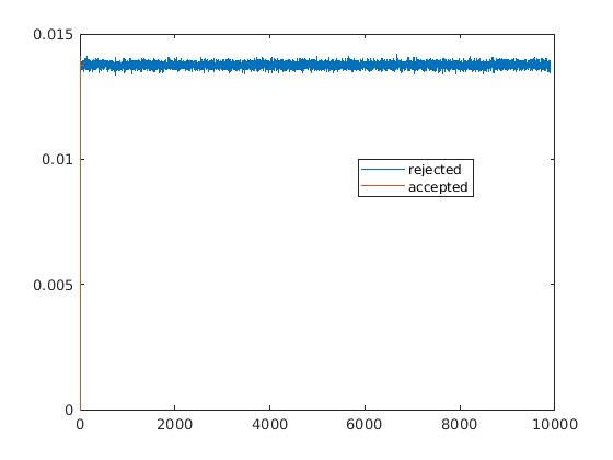
I start with a very big proposal standard deviation (E.sig in the code as 50000). The problem is that if I run $10000$ iterations, only a very few samples are accepted like only $10$. It doesn't converge. As the E.sig is super high, does it take a long time to converge? If you see the rejected values, it seems to oscillate at some point with a constant mean and feels like it is stuck at a local minima probably?

The plot of accepted and rejected values are shown below. Here, the accepted values are only 12 so they are not visible. The pattern for the rejected values kind of gives an impression that it is unable to reach a good value for $u$. So, I feel the final value of accepted values could be a local minima and getting out of this point is harder for the algorithm. I have put a histogram of rejected and accepted values as well. The final value of $u$ is $6.26 \times 10^{4} $ and it occurs at iteration number $4878$ which is much before $10000$.

enter image description here enter image description here enter image description here

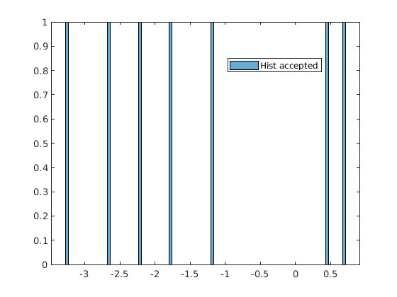
Next I show a case with E.sig = 1. However, in a practical scenario, one would like to start at a higher value. Is there a way to avoid this? Here also the acceptance rate is so low (only 10 out of 10000).

enter image description here enter image description here enter image description here

UPDATE: With answer 2

I have tried the values of the second answer.

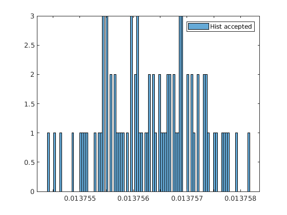
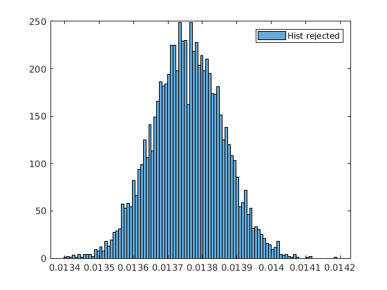
$\lambda = 1$, $u_{true} = 0.01$, $\sigma_n^2 = 0.01$, $dt = 0.1$. Start value of $u_{start} = 0.014$ and the proposal distribution of $u$ has a standard deviation of $u_{std} = 0.0001$. The results are below.

enter image description here enter image description here enter image description here

I have $110$ accepted values out of a $10000$ iterations.

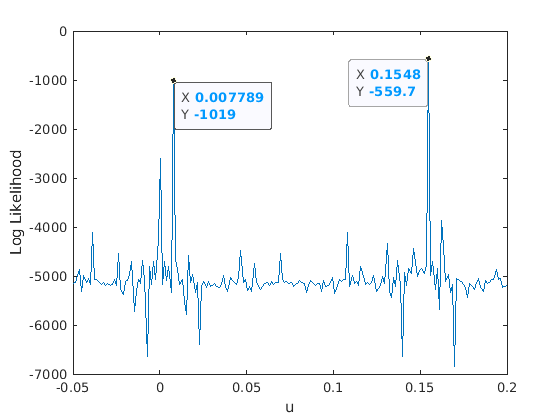
I also plot a likelihood in log for various values of $u$ as in the second answer. It looks similar but not smooth.

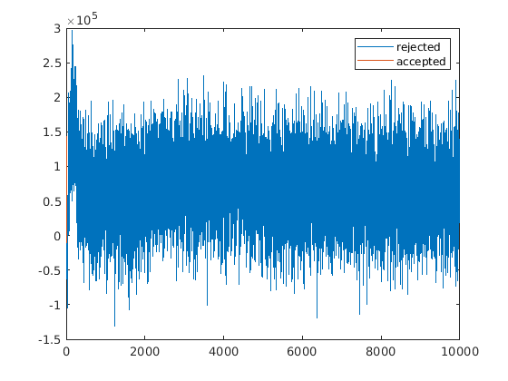
enter image description here

$\endgroup$
20
  • 4
    $\begingroup$ It would be better if you would provide a complete reproducible example. There are currently several problems and it is unclear whether these are the cause of the problems with convergence. Examples of unclear cases is why you do not simply multiply the likelihood functions since the noise terms are independent $p(a,b) = p(a)p(b)$. Then you will have one single comparison with the rand instead of two. $\endgroup$ Commented Apr 20, 2022 at 9:45
  • 2
    $\begingroup$ Another thing is that the real and imaginary parts of $\log(p(z|u))$ is not the same as using the real and imaginary parts for $z$ and $x$. $$\log(p(z|u))_{real} \neq \log(p(z_{real}|u))$$ $\endgroup$ Commented Apr 20, 2022 at 9:50
  • 2
    $\begingroup$ "It is actually reproducible" I can not reproduce this problem. Your example doesn't provide enough information for that. $\endgroup$ Commented Apr 20, 2022 at 10:33
  • 2
    $\begingroup$ ...to avoid all these sorts of confusion it is better if you include the entire procedure and something that can be reproduced by others. At the moment we keep making slow steps based on tiny errors and there is no complete overview of what you are doing. $\endgroup$ Commented Apr 20, 2022 at 11:51
  • 1
    $\begingroup$ I have gone through your code now and I have a good idea what can be going one. I want to write an answer similar to LudvigH's answer and my earlier comment about the problem of fitting a wave function. In order to make my answer stay close to your situation I am wondering how you are updating E.sig. Your histogram shows proposals in the order of $10^5$ which is due to that large E.sig and that, of course, results in a lot of rejections because you are sampling in a region with low probability density. (with a smaller E.sig the problem will be different). $\endgroup$ Commented Apr 22, 2022 at 10:08

2 Answers 2

2
+50
$\begingroup$

It is hard to tell if your problem is due to mistakes inyour implementation or if it is about the actual estimation problem. We don't have any working code to inspect. I implemented a working example for you -- see code below. I have also made an analysis of your problem, as described below.

The code implements Metropolis-Hastings with Brownian motion proposal. I tinkered quite some time with initialization and step size. The solution is very much dependant on these values. In the code, they are called u and step size. The values in the code currently comes from a kind of manual annealing burn in -- I started with a wild guess for u and large step_size. At the end of that run, I wrote down the final u, and restarted the whole process at that u, but with smaller step_size. And repeated again and again. In the early runs, the acceptance rate is ca 0.5%. By the end, it is ca 50%. Reducing the step size further makes the samples autocorrelated, so I stopped here with the parameters in the code below.

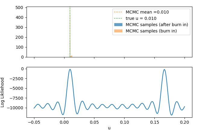
The reason why this kind of annealing scheme is needed is because of the nasty periodic structure of the likliehood with sharp local maxima. I plotted the log likelihood and the histogram of samples to illustrate that. The histogram is extremely narrow and quite hard to see in the plot using this axis limits, but quite nice to work with interactively. enter image description here

If the step size is too large, it will propose in the low-likelihood regions too often and get rejected. If the step size is too small, it get stuck in one of the small "bumps". The periodicity of the plot is due to aliasing. Run the code with differenet initializations and zoom around, and I think you will get a nice feel for it. :) I also played around with different noise levels, sample sizes, prior parameters etc. The conclusions changes with that of course. But in this low noise setting I have in the code below, the prior don't matter at all.

N.B. The plot shows the log likeliehood, since we are working with really small likelihoods. The use of logarithms can be crucial to get numerical stability.

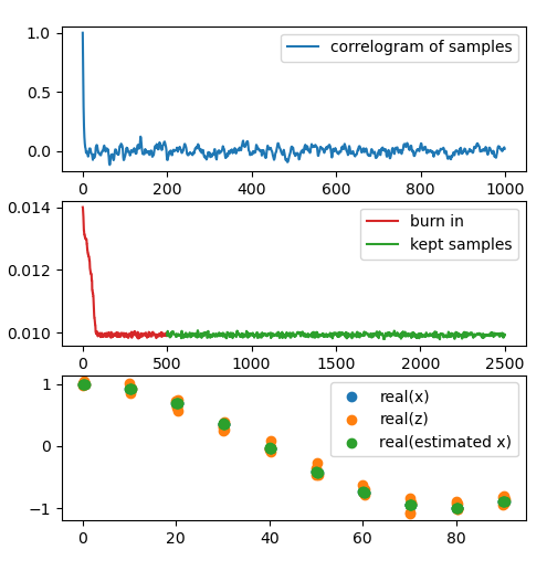
The code also produces a different diagnostic plot output plots. sharp histogram. low autocorrelation. quick burn-in. reasonable predictions

that tells us that the burn in period is long enough, that the autocorrelation between samples (after burn-in) is low, and that when I pick the expected posterior parameter, and generate synthetic data with it, it looks quite okay.

import numpy as np
import matplotlib.pyplot as plt

np.random.seed(999)


#
# Generate data for the observed time indices
#
dt = 0.1
M = 5
N = 100
u_true = 0.01 # the true u-value, to be estimated
lamda = 1 # assumed known
noise_variance = 0.01 # assumed known
t = np.array([N*k*dt + i*dt for i in range(5) for k in range(10)])
n_data = len(t)
x = np.exp(u_true*1j*t*4/lamda)
n = (
        np.random.standard_normal(size=n_data) +
        1j*np.random.standard_normal(size=n_data)
    )*np.sqrt(noise_variance)/np.sqrt(2)
z = x + n

#
# Configure and Initialize Metropolis-Hastings
#
sigma2_u = 1 # the variance of the gaussian prior
mu_u = 0     # the mean of the gaussian prior
proposal_step_size = 0.0001  # adjusted in manual "annealing" process
u = 0.014                    # initialization
get_proposal = lambda u:  u+np.random.standard_normal()*proposal_step_size # proposal is brownian motion
burn_in_samples = 500
mcmc_steps = burn_in_samples+ 2000

def log_proposal_density_ratio(u_new,u):
    """The proposals density is symmetric, so the ratio is always 1, and the log(1) = 0 always"""
    return 0

def log_likeliehood(u):
    """ compute the log likeliehood of this parameter
    as in
        log(p(z,u)) = log(p(u)) + log(p(z|u))   
    """
    x = np.exp(u*1j*t*4/lamda) #compute the predicted data sequence under this u
    n = z - x                  # compute the observed noise, assuming this predicted sequence
    n_real_std = np.real(n) * np.sqrt(2) / np.sqrt(noise_variance) # this is a vector of standard-normal distributed values, under the model assumptions
    n_imag_std = np.imag(n) * np.sqrt(2) / np.sqrt(noise_variance)
    ll1 = -0.5*np.log(2*np.pi) - 0.5*n_real_std**2                 # this is a vector of log likliehoods per observation
    ll2 = -0.5*np.log(2*np.pi) - 0.5*n_imag_std**2
    log_p_z_given_u = ll1.sum() + ll2.sum()
    log_p_u = -0.5*np.log(2*np.pi*sigma2_u)-0.5*(u-mu_u)**2/sigma2_u
    return log_p_u+log_p_z_given_u


#
# Run Metropolis-Hastings Algorithm
#
ll = log_likeliehood(u)
us = np.zeros(mcmc_steps)
did_accept = np.zeros(mcmc_steps)
for step in range(mcmc_steps):
    u_new = get_proposal(u)
    ll_new = log_likeliehood(u_new)
    accept_ratio = np.exp(ll_new - ll + log_proposal_density_ratio(u_new,u))
    rand = np.random.random()
    if rand < accept_ratio:
        u = u_new
        ll = ll_new
        did_accept[step] = 1
    else:
        did_accept[step] = 0

    us[step] = u

#
# Do diagnostics on the results
#
print(f"After burn in, {did_accept.mean():.1%} of the proposals were accepted.")
print(f"There are {len(np.unique(us[burn_in_samples:]))} unique values in the kept samples")

fig,axs = plt.subplots(3,1,figsize=plt.figaspect(1))
axs=axs.flatten()
variation = us[burn_in_samples:]-us[burn_in_samples:].mean()
variation /= np.linalg.norm(variation)
corrs = np.correlate(variation,variation,mode='same')
axs[0].plot(corrs[len(corrs)//2:],label='correlogram of samples')
axs[0].legend()
axs[1].plot(np.arange(burn_in_samples),us[:burn_in_samples],color='C3',label='burn in')
axs[1].plot(np.arange(burn_in_samples,mcmc_steps),us[burn_in_samples:],color='C2',label='kept samples')
axs[1].legend()
axs[2].scatter(t,np.real(x),label='real(x)')
axs[2].scatter(t,np.real(z),label='real(z)')
axs[2].scatter(t,np.real(np.exp(us.mean()*1j*t*4/lamda)),label='real(estimated x)')
axs[2].legend()


#
# Explanation plot
#
urange = np.linspace(-0.05,0.2,500)
lls = np.array([log_likeliehood(u) for u in urange])
fig,axs = plt.subplots(2,1,sharex=True)
axs=axs.flatten()
axs[0].hist(us[burn_in_samples:],label='MCMC samples (after burn in)',alpha=0.7)
axs[0].hist(us[:burn_in_samples],label='MCMC samples (burn in)',alpha=0.5)
axs[0].axvline(us.mean(),label=f'MCMC mean ={us.mean():.3f}',color='C1',linestyle='dotted')
axs[0].axvline(u_true,label=f'true u = {u_true:.3f}',color='C2',linestyle='dotted')
axs[0].legend()
axs[1].set_ylabel("Log Likliehood")
axs[1].set_xlabel("u")
axs[1].plot(urange,lls)
plt.show()

In summary:

  • I can't tell from your description if you had any problems with the implementation. It seems from the discussion with Sextus Empiricus that there might be misundrestanding about how to compute the likeliehood.
  • Metropolis Hastings can be used on this problem to generate samples from the posterior, if appropriate step size is used and it is initialized around a suitable local optimum.
  • The use of logarithms may be critical, as log likelihoods can be as small as -2500 .
  • For my number of data points and noise levels, the prior didn't have any notice'able effect. It can matter in your case.
$\endgroup$
8
  • $\begingroup$ Thank you for the detailed answer. I will change my question clearly again with a working example. $\endgroup$
    – CfourPiO
    Commented Apr 21, 2022 at 7:44
  • 1
    $\begingroup$ Thank you for adding a working example. It seems you have some minor mistakes (e.g. you double count the effect of the prior, you don't generate data as described in the question etc) but I think the MH implementation is ok. $\endgroup$
    – LudvigH
    Commented Apr 21, 2022 at 12:49
  • 1
    $\begingroup$ So I really don't have much more to add to the answer than what I already gave. The Log Liklelihood is super rugged, and a brownian motion proposal will only work for tiny step sizes. $\endgroup$
    – LudvigH
    Commented Apr 21, 2022 at 12:50
  • 1
    $\begingroup$ I had one more doubt. The proposal_step_size and sigma2_u are two different things in your code? Why is so? I thought the values of $u$ that is tested in the MCMC algorithm should come from a distribution like the prior. You have chosen a distribution, but you are not testing many values from that distribution. You are only checking with a very small width. $\endgroup$
    – CfourPiO
    Commented Apr 21, 2022 at 13:39
  • 1
    $\begingroup$ the prior (you stated in the question it is gaussian) is part of the bayesian methodology. the proposal distribution comes from the MH algorithm, and you can use MH as a frequentist or in a bayesian way. I suggest you read and do exercises from stat.columbia.edu/~gelman/book/BDA3.pdf to learn more. $\endgroup$
    – LudvigH
    Commented Apr 22, 2022 at 7:13
3
$\begingroup$

If I try to reproduce the data I get this as the sample:

data

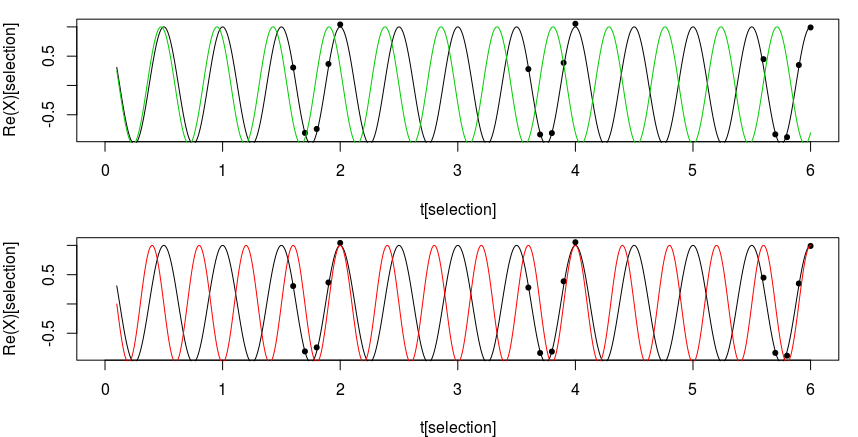
Because these are many cycles (1000), the fitting of this with a wave function requires a very small margin of error in the parameter $u$. When a small difference is made, then this has already a large influence on the position after 1000 cycles.

Below you see this with an example where every 20 time-ticks a sample of 5 is taken. In the first image with the green curve the frequency is changed by a factor 5% and this has little effect for small times $t$ on the left but a large effect on the right.

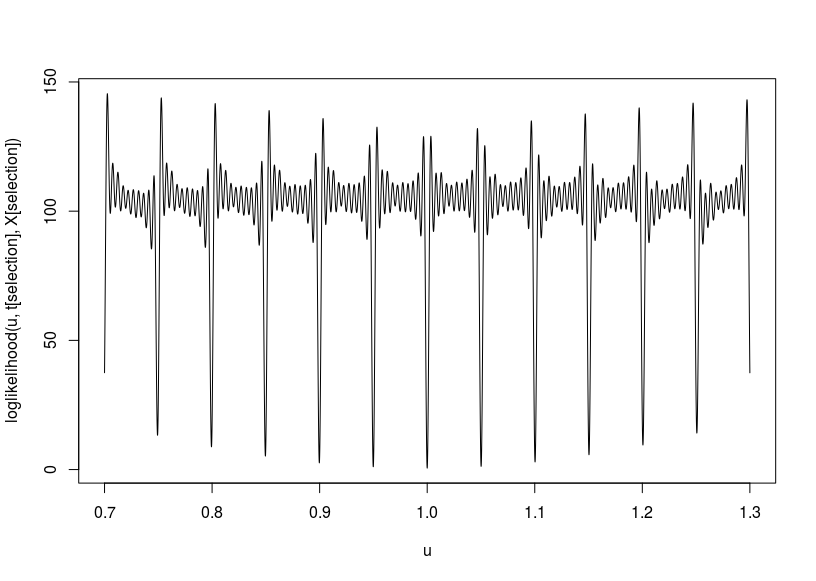
For a few special ratios in the frequency, like 1.25, which is the red curve below in the second image, some of the points in the wave function coincide and you get a relatively higher likelihood. This makes that you get multiple peaks in the likelihood function.

example of increasing error

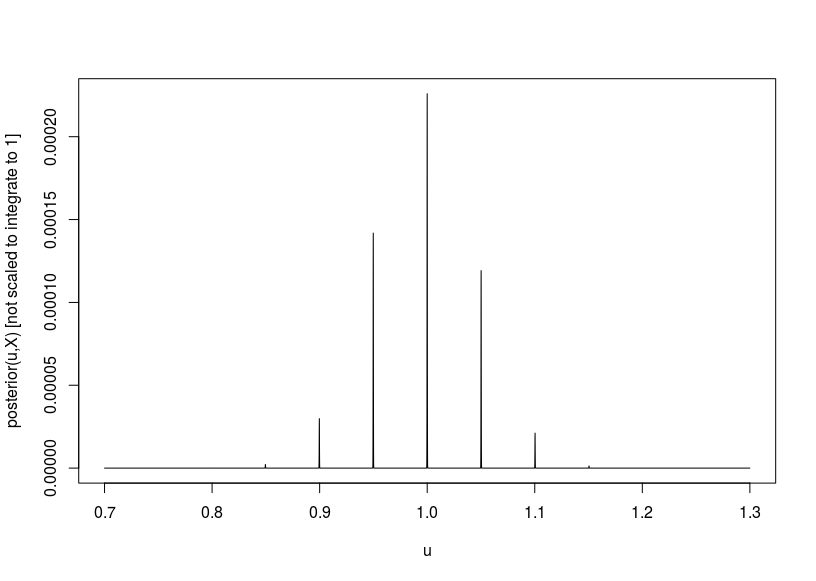
The consequence is a likelihood and prior that is very sharp.

likelihood

posterior

Your proposal function has a much wider range and so you are gonna sample mostly in the region with non-zero probability. What you need is a first good estimate of the $u$ and the bandwidth of the prior. Then you can get a better function that proposes new samples within the range.


Is still have to make the MCMC part for this question, but how do you compute the prior? I can not find this easily in your code. You have this function function ret = acceptance(u, u_new) but it seems to compare exp(u_new - u), which is the likelihood ratio but not the ratio of the posterior.


It might possibly be easier to use the variable $X(t)-X(t-1)$ (and since you observe batches of 5 consecutive times you get batches of 4 of those differences). Then you get that a small change in $u$ has not such a large effect on the likelihood. It may also be more realistic in cases that are not so steady. With your current likelihood function you are saying that the ground truth $e^{iu4\pi/\lambda t}$ has no variability after hundreds of cycles and that the process is very steady. So currently you assume that the error distribution is the same after hundreds of seconds as after 1 second.


R-code

######
######

set.seed(1)
### Parameters for sampling
###
### Nt = N*S numbers are the ground truth
### every N numbers there are M numbers sampled
N = 100
M = 5  
S = 10   
Nt = N*S

### Parameters for signal
dt = 0.1
u = 1
lambda = 1

### Parameters for noise
SNRdb = 20
SNR = 10^(SNRdb/10)
sigma = 1/sqrt(SNR)


### create variables

t = c(1:Nt)*dt            ### time variable
Z = exp(1i*4*pi/lambda*u*t) ### signal
sigma = sqrt(sum(abs(Z)^2)/(Nt * SNR)) 
epsilon = 1/sqrt(2) * (rnorm(Nt, 0, sigma) + 1i * rnorm(Nt, 0, sigma))   ### noise
X = Z + epsilon
selection = rep(N*c(1:S),each = M) + rep(1:M,S) - M ### id's of S times M consequitve id's with gaps of N

plot(X) ### view the variable

loglikelihood = function(uf,t,X) {
 x_fit = exp(1i*4*pi/lambda*uf*t)
 residual = x_fit-X
 error = sum(Im(residual)^2 + Re(residual)^2)
 return(error)
}
loglikelihood = Vectorize(loglikelihood, "uf")

posterior = function(uf,t,X) {
  prior = dnorm(uf,1.3,10^3)
  exp(-1*loglikelihood(uf,t,X))*prior
}
posterior = Vectorize(posterior, "uf")


u = seq(0.7,1.3,0.0001)
plot(u,loglikelihood(u,t[selection],X[selection]), log = "", type = "l")


u = seq(0.7,1.3,0.00001)
plot(u,posterior(u,t[selection],X[selection]), log = "", type = "l",
     ylab = "posterior(u,X) [not scaled to integrate to 1]")
$\endgroup$
7
  • $\begingroup$ Thanks for the answer. What I do here is that I treat the real part and imaginary part separately for the likelihood function. So, $K$ is also used separately twice. I think only by taking the real part of the signal, I can do the analysis without bothering about the imaginary part. The noise variance is the same for the real and imaginary parts. $\endgroup$
    – CfourPiO
    Commented Apr 19, 2022 at 11:49
  • $\begingroup$ Is it a good idea to look for complex normal distribution? Can it use the complex signals as it is to find a likelihood at the end? $\endgroup$
    – CfourPiO
    Commented Apr 19, 2022 at 11:50
  • $\begingroup$ @CfourPiO the complex normal distribution of the complex n-vector $z$ is equivalent to a multivariate normal distribution of the real 2n-vector $Re(z), Im(z)$ (the other way around is not true in general). So you do not really need to use the complex normal distribution. Possibly it might be convenient for your case if you want to describe a particular correlation structure. $\endgroup$ Commented Apr 19, 2022 at 16:07
  • 1
    $\begingroup$ I am deleting this answer for the moment. I placed this answer because your likelihood function already looked very weird and seemed to be at least some problem (with the imaginary part). Could you clarify in more detail the steps that you took. It is difficult to reproduce your problem. For instance it is not clear how you computed the likelihood exactly and which MCMC method you used or what software and function call you used and in what way you compute the proposals for new draws (e.g. a problem is if your proposal function is very different from the posterior that you try to sample from). $\endgroup$ Commented Apr 19, 2022 at 16:23
  • 2
    $\begingroup$ You could tackle this problem with some manual work, but if you are looking for some very reliable and effective code to tackle this situation automatically, then you could search for some fancy proposal function that is a Gaussian mixture of three normal distributions and has three modes. One central mode that makes the sampling within the peaks, and also a mode at plus 5% and a mode at minus 5%, which ensure that you don't get stuck in a local optimum. $\endgroup$ Commented Apr 25, 2022 at 9:04

Your Answer

By clicking “Post Your Answer”, you agree to our terms of service and acknowledge you have read our privacy policy.

Not the answer you're looking for? Browse other questions tagged or ask your own question.