I have a question regarding survival analyses: Imagine I have a large cohort, where most participants have been given one treatment (treatment A), and a much much smaller subpopulation which has been given another treatment (say, treatment B). We follow both groups for 5 years. In group receiving treatment B, no one dies. In group A, 10% die. Now, there are obvious potential issues here around bias and sampling that could be going on. But let's say both groups are well-matched, apart say for one or two covariates. What method would be best to get some insight into whether treatment B may actually be superior, or if it's just a sampling effect or something else going on, particularly given the small sample size of group B? Thank you!
-
$\begingroup$ Did you measure/record the one or two covariates that might affect survival and are different between groups? $\endgroup$– dipetkovCommented Apr 21, 2022 at 21:50
-
$\begingroup$ @dipetkov Yes I did, thank you! $\endgroup$– hyst111Commented Apr 21, 2022 at 22:16
1 Answer
If you don't have to correct for covariates, then you can evaluate the difference with a standard log-rank test. See this answer.
If you are doing Cox modeling to control for covariates, the Wald test typically reported on the coefficient for the treatment will be useless. Therneau and Grambsch discuss this situation in Section 3.5, "Infinite Coefficients," of Modeling Survival Data--Extending the Cox Model, and use the following (contrived) example that is sure to lead to an infinite coefficient:
library(survival)
fit <- coxph(Surv(futime, fustat) ~ rx +
           fustat, ovarian)
## warnings not shown here
summary(fit)
# Call:
# coxph(formula = Surv(futime, fustat) ~ rx +
   fustat, data = ovarian)
#
#   n= 26, number of events= 12
#
#              coef  exp(coef)   se(coef)      z Pr(>|z|)
# rx     -5.566e-01  5.731e-01  6.199e-01 -0.898    0.369
# fustat  2.258e+01  6.414e+09  1.387e+04  0.002    0.999
#
#        exp(coef) exp(-coef) lower .95 upper .95
# rx     5.731e-01  1.745e+00      0.17     1.932
# fustat 6.414e+09  1.559e-10      0.00       Inf
#
# Concordance= 0.897  (se = 0.037 )
# Likelihood ratio test= 30.8  on 2 df,   p=2e-07
# Wald test            = 0.81  on 2 df,   p=0.7
# Score (logrank) test = 29.09  on 2 df,   p=5e-07
They say:
We do not view this as a serious concern at all, other than an annoying numerical breakdown of the Wald approximation. One is merely forced to do the multiple fits necessary for a likelihood ratio or score test.
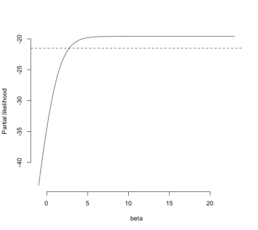
I think that the likelihood-ratio test for individual coefficients is implemented directly in SAS. With R, you can examine the log-likelihood as a function of treatment-coefficient values beta (the profile likelihood) as Therneau and Grambsch outline in Section 3.4.1:
...first fit the overall model using all covariates...then [fit] a sequence of Cox models. For each trial value of
beta, an offset term is used to includebeta * [your treatment indicator]in the model as a fixed covariate. This essentially fixes the coefficient at the chosen value, while allowing the other coefficients to be maximized.
Here's how to do this for their contrived example:
beta <- seq(-1,23,length=500)
llik <- double(500)
for (i in 1:500) { temp <- coxph(Surv(futime,
    fustat) ~ rx + offset(beta[i]*fustat),
    data=ovarian);llik[i] <- temp$loglik[2]}
## There were 50 or more warnings (use
## warnings() to see the first 50)
plot(beta, llik, type="l",
     ylab="Partial likelihood", bty="n")
temp <- fit$loglik[2] - qchisq(0.95,1)/2
       ## for 95% CI
abline(h=temp,lty=2)
For the intersection point:
beta[which.min(abs(llik-(fit$loglik[2]
     -qchisq(0.95,1)/2)))]
## [1] 2.751503
So the 95% CI for the Cox regression coefficient would be 2.75 to infinity.
Whether you are using a log-rank test without covariate adjustment or a Cox model with it, repeat the modeling and analysis on multiple bootstrapped samples of your data to evaluate the robustness of the result.

