How are sums and differences of independent Exponential random variables distributed?

Question

If we are given X₁, X₂, X₃, X₄ , all exponential random variables with the same mean λ and said that another random variable T = X₁ + X₂ + X₃ - X₄. Can we then say T basically has a Gamma Distribution with parameters (2,λ)? I know we can sum up exponentials and obtain a gamma; however, I wonder if we can apply the same logic for subtraction. I think it is possible considering these random variables as arrivals to a Poisson Process, nevertheless I wanted to ask.

Answer 1

Because the characteristic function of an exponential distribution is

$$\phi(t) = \frac{1}{1 - it},$$

when $X_1,\ldots, X_4$ are independent exponentially distributed variables (all with the same rate, which with no loss of generality may be taken as unity), the characteristic function of $X = X_1+X_2+X_3-X_4$ is

$$\phi_X(t) = \phi(t)^3\phi(-t) = \frac{1}{(1-it)^3(1+it)}.$$

Using partial fractions this is easily decomposed and inverted (by inspection or direct calculation of the inverse Fourier transform) to give the density

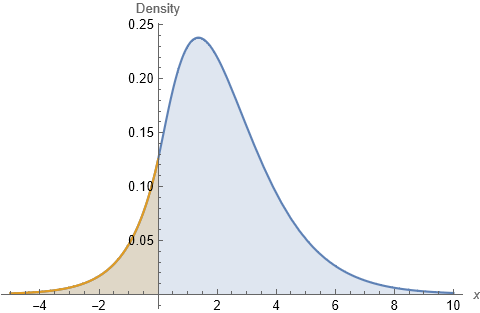
$$f_X(x) = \frac{1}{8} \left(e^{x} \mathcal{I}(x\le 0) + e^{-x}(1 + 2x + 2x^2)\mathcal{I}(x\gt 0)\right).$$

This is recognizable as a mixture of a Laplace distribution, a Gamma$(2)$ distribution, and a Gamma$(3)$ distribution.

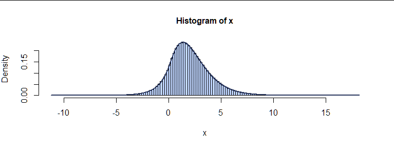
As a check, in R I generated a million independent $(X_1,X_2,X_3,X_4)$ tuples and plotted this histogram of $X_1+X_2+X_3-X_4$ to compare it to the graph of $f_X,$ as shown.

hist(c(1,1,1,-1) %*% matrix(rexp(1e6*4), 4), freq=FALSE, breaks=200, xlab="x", main="")
curve(1/8 * (dgamma(-x, 1) + dgamma(x, 1) + 2*dgamma(x, 2) + 4*dgamma(x, 3)))

The agreement is excellent.

---

Generalization

Because the question refers to "sums and differences" quite generally, I thought it might be interesting to obtain a general answer. To that end, note that the characteristic function (cf) of the sum of $k$ iid minus the sum of $j$ iid exponential variables will be

$$\phi_{k,j}(t) = (1 - it)^{-k}(1 + it)^{-j}.$$

The aim is to express this, if possible, as a mixture (linear combination) of Gamma cfs. Recall that a Gamma distribution with shape parameter $\alpha$ has $(1-it)^{-\alpha}$ for its cf. It is immediately apparent that $\phi_{k,j}$ is the cf for the difference of a Gamma$(k)$ and (independent) Gamma$(j)$ variable. But that doesn't get us any further towards a solution.

This problem turns out to be purely algebraic. Upon writing

$$a = \frac{2}{1-it},\quad b = \frac{2}{1+it},$$

observe that $1/a + 1/b = 1,$ whence $a + b = ab.$ Our objective, then, can be attained if we can express $a^k b^j$ as a linear combination of pure (positive) powers of $a$ and $b.$ (Formally, the calculations are done in the polynomial quotient ring $\mathbb{Q}(a,b)/(a+b-ab).$ No analytic considerations of convergence, etc., will be needed.)

The idea is to find $a^kb^j$ recursively.

• The base case is $a^k=a^k:$ we already have a pure power of $a.$

• The next case is $$a^kb = a^{k-1}(ab) = a^{k-1}(a+b) = a^k + a^{k-1}b.$$ So, if $k\gt 1,$ repeat this process, ultimately finding $$a^kb = a^k + a^{k-1} + \cdots + a^2 + a + b.$$

• The next step shows us what will happen generally, using the preceding result to expand each of the terms that appears in the final multiplication by $b$: $$\begin{aligned} a^k b^2 &= (a^k b)b = \left(a^k + a^{k-1} + \cdots + a^2 + a + b\right)b\\ &= a^kb + a^{k-1}b + \cdots + a^2b + ab + b^2\\ &= a^k + a^{k-1} + \cdots + a^2 + a + b\\ &+ \quad a^{k-1} + \cdots + a^2 + a + b\\ &\cdots\\ &+ \quad\quad\quad (a+b) + b^2\\ &= \left(a^k + 2a^{k-1} + \cdots + ka\right) + \left(k b + b^2\right). \end{aligned}$$

Proceeding in this vein, we arrive at a general formula (which is easily proven inductively):

$$a^k b^j = \sum_{i=1}^k \binom{k+j-1-i}{j-1} a^{i}\ +\ \sum_{i=1}^j\binom{k+j-1-i}{k-1} b^{i}.$$

(That's rather a pretty relation in its own right...)

Upon dividing both sides by $2^{k+j}$ and re-expressing $a$ and $b$ in terms of $t,$ we obtain the desired decomposition, from which we may read off the Gamma shape parameters and mixture weights directly:

$$\phi_{k,j}(t)=\sum_{i=1}^k \binom{k+j-1-i}{j-1}2^{i-j-k} \phi(t)^i\ +\ \sum_{i=1}^j\binom{k+j-1-i}{k-1} 2^{i-j-k} \phi(-t)^i.$$

For example, the combination in the question corresponds to a sum of $k=3$ exponentials minus $j=1$ exponential, for which

$$\begin{aligned} \phi_{3,1}(t) &= \binom{3-1}{0}2^{1-4}\phi(t)+\binom{3-2}{0}2^{2-4}\phi(t)^2+\binom{3-3}{0}2^{3-4}\phi(t)^3\\&\quad+ \binom{1-1}{0}2^{1-4}\phi(-t)\\ &= \frac{1}{8}\phi(t)+\frac{1}{4}\phi(t)^2+\frac{1}{2}\phi(t)^3+\frac{1}{8}\phi(-t), \end{aligned}$$

telling us the distribution is a mixture of $1/8$ exponential, $1/4$ Gamma$(2),$ $1/2$ Gamma$(3),$ and $1/8$ reversed exponential distributions.

Here is an R implementation modeled on the previous code. It also includes a common rate parameter for all the exponentials. (It played no role in the calculations because it merely establishes a common unit of measurement for all the distributions.)

#
# Density of the sum of `k` and difference of `j` *iid* exponentials.
# (Equivalently, the difference of a Gamma(k) and Gamma(j) distribution.)
#
f <- Vectorize(function(x, k, j, ...) {
  g <- function(x, k, j) {
    i <- seq_len(k)
    sum(choose(k+j-1-i, j-1) * 2^(i-j-k) * dgamma(x, i, ...))
  }
  g(x, k, j) + g(-x, j, k)
}, "x")
#
# Simulated data.
#
k <- 9
j <- 4
rate <- 10
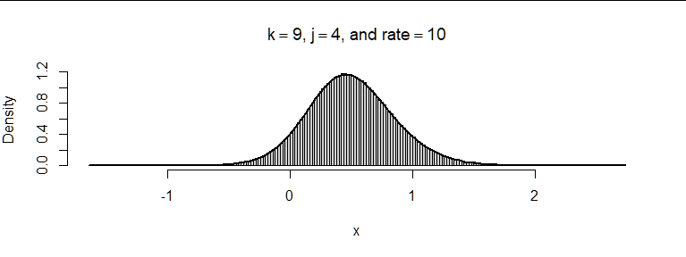
hist(c(rep(1,k), rep(-1,j)) %*% matrix(rexp(1e6 * (k+j), rate), k+j), 
     freq=FALSE, breaks=200, xlab="x", 
     main=bquote(paste(k==.(k), ", ", j==.(j), ", and rate"==.(rate))))
#
# Check by overplotting the density function.
#
curve(f(x, k, j, rate=rate), add=TRUE, lwd=2)

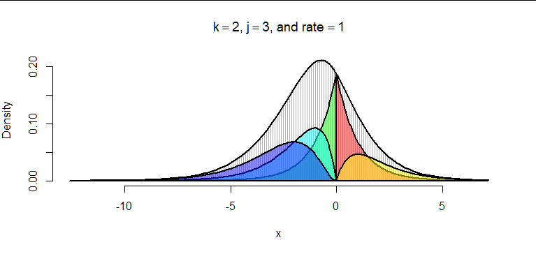
The positive components will have Gamma distributions with shape parameters $1, 2, \ldots, k$ while the negative components, when reversed, will have Gamma distributions with shape parameters $1,2,\ldots, j.$ As an illustration the next histogram, produced by the preceding code, also displays the components, suitably weighted and color-shaded to differentiate them. Their sum is plotted in black, nicely tracing out the histogram.