How to interpret angles between explantory variables in Redundancy analysis (RDA)?

Question

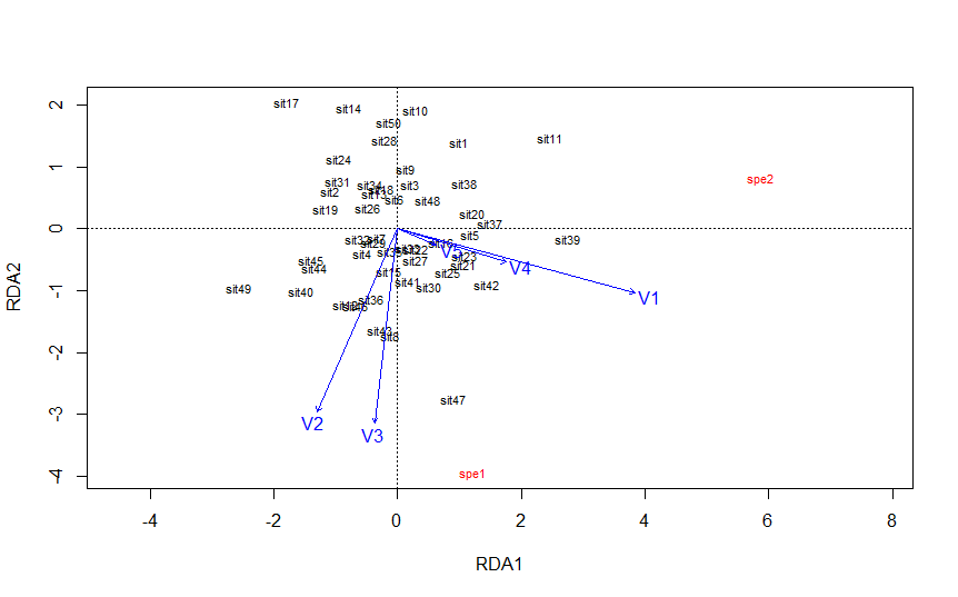
I am learning to apply constrained ordination to community data using the vegan package in R. According to some materials, like this one, in a scaling type 2 RDA triplot:

Angles between all vectors reflect linear correlation.

It confuses me how the triplot would look like if all explanatory variables are uncorrelated. I tested in R by creating a matrix consists of 5 vectors with very low（0.001）correlations (code copied from the second answer) as explanatory variables, and two artificial response variables like below :

set.seed(42)
require(vegan)

# generate uncorrleated variables
n <- 5

R <- matrix(.001, nrow = n, ncol = n)
diag(R) <- 1

# Cholesky decompostion of correlation matrix
Lut <- chol(R)
L <- t(Lut)

# Standard deviations
sds <- seq(10, 1, length.out = n)

# VCOV matrix
Sigma <- diag(sds) %*% L %*% Lut %*% diag(sds)

# Generate variables
library(MASS)
X <- mvrnorm(50, mu= rep(0, n), Sigma, empirical = TRUE)
cor(X)

#generate response variables
b1=c(0.2,0.3,0.5,0.3,0.4)
b2=c(0.5,-0.3,-0.2,0.7,0.8)
y1=b1%*%t(X)+rnorm(10,sd=0.01)
y2=b2%*%t(X)+rnorm(10,sd=0.01)

#do RDA
y=cbind(as.vector(y1),as.vector(y2))
X=as.data.frame(X)
rd=vegan::rda(Y=X,X=y)
plot(rd,scaling=2)

And it generates plot like this, with V1, V4 and V5 very close to each other though they have low correlations.

So my question is what is wrong with my understanding and how should I interpret angles between explanatory vectors in a RDA triplot?

Answer 1

You had two variables in your response matrix y. So it has rank=2 and can be expressed by any two explanatory variables. You had five explanatory variables, or three extra. You would need 5-dim space to draw them all perpendicular to each other, but you only have 2 dims. Anyway, the arrows are in two bunches, and these bunches are perpendicular to each other. Moreover, if you pick any two X-variables, they will look uncorrelated to each other (at 90 degrees). Try several times

plot(rda(y, X[, sample(5,2)]), scaling=2)

However, if you pick three variables, one of them cannot be perpendicular to two others, as there is no third dimension to go. So it must be in the same bunch with one of those two. Again, try several times

plot(rda(y, X[, sample(5,3)]), scaling=2)

The same applies to all 5 of your X.

You need more dimensions. That is, more columns in y. Naturally, you still see only 2-dim projections of those arrows in 5-dims, but probably more or less evenly spread with angles as close to 90 degrees as you can have for five arrows in 2 dim. Looking at 5-dims is hard, but there they are like you assume: perpendicular to each other.