I've constructed a logistic glmm for predicting if individuals of a single species of fish caught will have an empty stomach or not (1=emtpy, 0=not empty). My predictor variables are salinity (sal), temperature (temp), standard length (SL), Station/location (which are not the same each year, but neither are they randomly chosen) and calendar year (CYR). I've modelled Station and CYR as random intercepts because, 1. They're both factors with many levels, and 2. (my hypothesis), the log-likelihood of a fish unsuccessfully catching something (correct to say?) depends on the prevailing conditions (presence of predators and prey, water quality, etc..) all change/depend on the location and year. So, hopefully I've got the random intercept correct.
Where I get confused is the logic for including random slopes and translating it to my scenario. This resource has been very helpful, but I'm not sure I have it right or how to "test" the idea/visualize including a random slope for logistic regression. My best guess is that the size of a fish (hence its age/experience) influences how good it is at seeking out and catching food, but that that also depends on the location and time. As in, maybe smaller fish stay in certain locations during different years based on changing conditions (hence a random slope)(?).
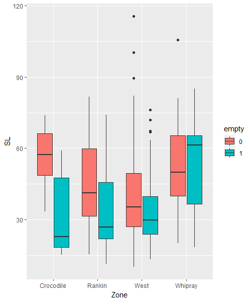
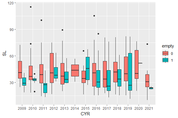
Plots:
(Many Stations make-up a "zone" and smaller fish (red boxplot with smaller median all have "non-empty stomachs) seem to eat better @ Whipray)
Would an ANOVA comparing mod1 and mod2 show which is better (random slope + intercept or just random intercept)? Any help interpreting the summary output as well is greatly appreciated! I'm not sure how to interpret the variance from the random effects or how to decide if my variables are too strongly correlated (or if it matters since 2/3 aren't significant). I also get an error for the more complicated model (mod2).
Only random intercepts:
mod1 <- glmer(empty ~ SL + sal + temp + (1 | CYR) + (1 | Station), family=binomial, data = c_neb, control=glmerControl(optimizer = "bobyqa"))
Random slopes and intercepts:
mod2 <- glmer(empty ~ SL + sal + temp + (SL | CYR) + (SL | Station), family=binomial, data = c_neb, control=glmerControl(optimizer = "bobyqa"))
Summaries:
  > summary(mod1)

Generalized linear mixed model fit by maximum likelihood (Laplace Approximation) ['glmerMod']
 Family: binomial  ( logit )
Formula: empty ~ SL + sal + temp + (1 | CYR) + (1 | Station)
   Data: c_neb
Control: glmerControl(optimizer = "bobyqa")

     AIC      BIC   logLik deviance df.resid
   757.6    784.8   -372.8    745.6      682

Scaled residuals:
    Min      1Q  Median      3Q     Max
-1.1509 -0.5940 -0.4666  0.8429  3.3439

Random effects:
 Groups  Name        Variance Std.Dev.
 Station (Intercept) 0.1986   0.4457
 CYR     (Intercept) 0.1249   0.3534
Number of obs: 688, groups:  Station, 90; CYR, 13

Fixed effects:
              Estimate Std. Error z value Pr(>|z|)
(Intercept)  0.6814783  1.1748120   0.580    0.562
SL          -0.0300014  0.0064659  -4.640 3.49e-06 ***
sal          0.0001171  0.0246037   0.005    0.996
temp        -0.0234828  0.0337120  -0.697    0.486
---
Signif. codes:  0 ‘***’ 0.001 ‘**’ 0.01 ‘*’ 0.05 ‘.’ 0.1 ‘ ’ 1

Correlation of Fixed Effects:
     (Intr) SL     sal
SL   -0.474
sal  -0.457 -0.011
temp -0.627  0.322 -0.367

##################################################################################################

> summary(mod2)

Generalized linear mixed model fit by maximum likelihood (Laplace Approximation) ['glmerMod']
 Family: binomial  ( logit )
Formula: empty ~ SL + sal + temp + (SL | CYR) + (SL | Station)
   Data: c_neb
Control: glmerControl(optimizer = "bobyqa")

     AIC      BIC   logLik deviance df.resid
   765.0    810.4   -372.5    745.0      678

Scaled residuals:
    Min      1Q  Median      3Q     Max
-1.0746 -0.5984 -0.4609  0.8671  3.1028

Random effects:
 Groups  Name        Variance  Std.Dev. Corr
 Station (Intercept) 3.057e-01 0.552944
         SL          1.020e-04 0.010101 -0.58
 CYR     (Intercept) 3.257e-02 0.180476
         SL          2.048e-05 0.004526 1.00
Number of obs: 688, groups:  Station, 90; CYR, 13

Fixed effects:
              Estimate Std. Error z value Pr(>|z|)
(Intercept)  0.5848489  1.2086079   0.484    0.628
SL          -0.0327655  0.0082548  -3.969 7.21e-05 ***
sal          0.0006626  0.0249615   0.027    0.979
temp        -0.0176335  0.0351176  -0.502    0.616
---
Signif. codes:  0 ‘***’ 0.001 ‘**’ 0.01 ‘*’ 0.05 ‘.’ 0.1 ‘ ’ 1

Correlation of Fixed Effects:
     (Intr) SL     sal
SL   -0.348
sal  -0.463 -0.021
temp -0.638  0.159 -0.340
optimizer (bobyqa) convergence code: 0 (OK)
boundary (singular) fit: see help('isSingular')


