Training on predicted labels for cross validation

Question

I've been training on predicted labels and then using that to predict the train data, using the resulting score as a measure of fitness of my model.

It seems to work quite well in many different scenarios, though I do notice that some level of accuracy is required otherwise the score can be a bit noisy and less useful.

I'd like to learn more about this technique. Does it have a name or are they any references I can check out to better understand what I'm doing? I'd like to use it for epoch selection, forward feature selection, hill climbing, etc.

Note that this technique isn't really cross validation in the sense of oof / folding. It's more inverting the prediction process and a semi supervised learning coherence process.

Also note that I'm not proposing using predicted labels for training, just for measuring model fitness. I find that can lead to overfitting, though I suppose so can what I'm suggesting, at least indirectly.

example code:

model_to_be_evaluated = LGBMRegressor()
model_to_be_evaluated.fit(Xtrain, ytrain)
SSL_model_evaluator = LGBMRegressor()
SSL_model_evaluator.fit(Xtest,model_to_be_evaluated.predict(Xtest))
score_for_model_to_be_evaluated = SSL_model_evaluator.score(Xtrain, ytrain)

The idea being that I'm trying to blend in information regarding the unlabeled test data and how they interact with the predictions. I see significant correlation in many scenarios (not all) with CV score / test scores.

In some situations, all you have are predicted labels. The correlation is generally perfect against scores on ground truth at a coarse enough level in most scenarios, which makes it useful for some purposes.

At the very minimum, I find it very useful as a quick sanity check.

edit to add that this might help with overfitting (Bjorn's point):

SSL_model_evaluator.score(Xtrain_holdout, ytrain_holdout)

Here is a complete code example using covtype dataset from sklearn (this is the first time I've tried this approach on this dataset):

import sklearn.datasets
cov = sklearn.datasets.fetch_covtype()

df = pd.DataFrame(cov.data)
df.columns = cov.feature_names
targ = 'Cover_Type'
df[targ] = cov.target
train = df.sample(frac=0.2).copy()
rest = df.drop(train.index).copy()
train_holdout = rest.sample(frac = 0.2).copy()
unlabeled = rest.drop(train_holdout.index).sample(frac=0.5)
for i in train, unlabeled, train_holdout:
    print(len(i))
len(train)+len(unlabeled)+len(train_holdout) == len(df)


import lightgbm, sklearn.model_selection, scipy.stats
X_holdout = train_holdout.drop(targ, axis = 1)
y_holdout = train_holdout[targ]
X = train.drop(targ, axis = 1)
y = train[targ]
X_test = unlabeled.drop(targ, axis = 1)
y_test = unlabeled[targ]
scs = []
for i in range(100, len(X), int(len(train)/20)):
    model = lightgbm.LGBMClassifier()
    #This is our model that we are evaluating
    model.fit(X[0:i],y.iloc[0:i])
    
    #Now we're going to distill knowledge from the unlabeled test set
    model_eval = lightgbm.LGBMClassifier()
    #We use the SSL pseudolabels to train with
    model_eval.fit(X_test,model.predict(X_test))
    #Loop multiple times on unlabeled test data for enhanced knowledge density
    for j in range(5):
        print(".", end="")
        model_eval1 = lightgbm.LGBMClassifier()
        model_eval1.fit(X_test,model_eval.predict(X_test))
        model_eval = lightgbm.LGBMClassifier()
        model_eval.fit(X_test,model_eval1.predict(X_test))
    #cv score for comparison
    cv_preds = sklearn.model_selection.cross_val_predict(lightgbm.LGBMClassifier(), X[0:i], y.iloc[0:i], cv=5, n_jobs=-1)
    roc = sklearn.metrics.accuracy_score(y.iloc[0:i], cv_preds)
    #This is our SSL metric
    v = sklearn.metrics.accuracy_score(y_holdout, model_eval.predict(X_holdout))
    #This is our ground truth score
    v2 = sklearn.metrics.accuracy_score(y_test, model.predict(X_test))
    print(i,v,v2, roc)
    scs.append([i, v,v2, roc])
    if len(scs) > 1:
        print("SSL Metric correlation", scipy.stats.pearsonr([x[1] for x in scs], [x[2] for x in scs]))
        print("CV correlation", scipy.stats.pearsonr([x[3] for x in scs], [x[2] for x in scs])) 
        print("CV + SSL correlation", scipy.stats.pearsonr([x[1]+x[3] for x in scs], [x[2] for x in scs])) 

df = pd.DataFrame(scs, columns = ["size", "SSL metric", "grnd score", "cv score"])
display(df.corr())
print("SSL Metric correlation", scipy.stats.pearsonr([x[1] for x in scs], [x[2] for x in scs]))
print("CV correlation", scipy.stats.pearsonr([x[3] for x in scs], [x[2] for x in scs]))





100 0.6066349691271702 0.6101848066952088 0.64
.....5910 0.7458746584625976 0.7838041350229126 0.7732656514382402
SSL Metric correlation (1.0, 1.0)
CV correlation (1.0, 1.0)
CV + SSL correlation (1.0, 1.0)
.....11720 0.7602138508207654 0.811412189927067 0.8033276450511946
SSL Metric correlation (0.9991068517535358, 0.0269084836575225)
CV correlation (0.9989002711826732, 0.029859170046122856)
CV + SSL correlation (0.9999959051170868, 0.0018218642469783922)
.....17530 0.7669800563671177 0.8208999376089154 0.8140901312036509
SSL Metric correlation (0.9989918045379589, 0.001008195462041117)
CV correlation (0.9983797333974359, 0.001620266602564091)
CV + SSL correlation (0.9999578462868633, 4.215371313665006e-05)
.....23340 0.7663776596889051 0.8284137604612637 0.8219794344473008
SSL Metric correlation (0.9976731160105244, 0.0001346927790430204)
CV correlation (0.998053283869585, 0.00010307680315341846)
CV + SSL correlation (0.9999315226935976, 6.802200040449242e-07)
.....29150 0.7730362943998623 0.8339751726511908 0.8266552315608919
SSL Metric correlation (0.997606186520421, 8.58865577639315e-06)
CV correlation (0.9979734083917876, 6.156448639323529e-06)
CV + SSL correlation (0.9999359217754913, 6.158896731084367e-09)
.....34960 0.77572556528474 0.8376110668875455 0.8301201372997712
SSL Metric correlation (0.9976059099140633, 5.379573298554177e-07)
CV correlation (0.9979292922627183, 3.743423127751737e-07)
CV + SSL correlation (0.9999368844933946, 6.078260889564408e-11)
.....40770 0.7685721047309654 0.839095544415998 0.8349766985528575
SSL Metric correlation (0.9956388999569111, 2.0668386326028505e-07)
CV correlation (0.9974544034623652, 4.1160363358897236e-08)
CV + SSL correlation (0.9998787077742654, 4.460662826642163e-12)
.....46580 0.7769518728082442 0.8406822142380758 0.8393945899527694
SSL Metric correlation (0.9957623303896034, 1.6243934882324038e-08)
CV correlation (0.9966095244747208, 7.447607149326285e-09)
CV + SSL correlation (0.9996882703419993, 1.7604708876086672e-12)
.....52390 0.7677760805490416 0.8430810438673867 0.8401221607176942
SSL Metric correlation (0.9930871025752668, 9.90857625137889e-09)
CV correlation (0.9962975371706202, 8.184836796820808e-10)
CV + SSL correlation (0.9995475274076026, 1.832784239150565e-13)
.....58200 0.7746068285966309 0.8350455024633722 0.8420274914089347
SSL Metric correlation (0.9931571058602614, 1.0513156735031128e-09)
CV correlation (0.9939105755200914, 6.226109128105513e-10)
CV + SSL correlation (0.9985711284072407, 9.204393460192126e-13)
.....64010 0.7840730621114004 0.838654503990878 0.8435713169817216
SSL Metric correlation (0.9920458296634339, 2.4743369407078367e-10)
CV correlation (0.9926253167154037, 1.6967659750598925e-10)
CV + SSL correlation (0.9971803735242705, 1.3969036471093728e-12)
.....69820 0.7679159226350551 0.8480830877132591 0.8407189916929246
SSL Metric correlation (0.9879449691152301, 2.907279904921447e-10)
CV correlation (0.9927929990874622, 1.7327452322624598e-11)
CV + SSL correlation (0.99621845913096, 5.024597051416664e-13)
.....75630 0.7756717798670425 0.8182214238075773 0.8436863678434484
SSL Metric correlation (0.9836951715303516, 2.6191890474789664e-10)
CV correlation (0.9833588368830564, 2.958397080779752e-10)
CV + SSL correlation (0.9892370594577319, 2.1930073622544316e-11)
.....81440 0.7792108603515415 0.8445171145199114 0.8405820235756385
SSL Metric correlation (0.9839456578957019, 4.102044996533527e-11)
CV correlation (0.9836510122857258, 4.613523813625284e-11)
CV + SSL correlation (0.9894169028452637, 2.7690159024078936e-12)
.....87250 0.7777801682407866 0.8465986101848066 0.845295128939828
SSL Metric correlation (0.9838842934546217, 7.255220825372512e-12)
CV correlation (0.9839113624449564, 7.1708579205882375e-12)
CV + SSL correlation (0.9895926542112893, 3.4500680328272935e-13)
.....93060 0.7733912781566662 0.8465502033088789 0.8463571889103804
SSL Metric correlation (0.9828849075303538, 1.964902980261665e-12)
CV correlation (0.9840779110411325, 1.1468137822713189e-12)
CV + SSL correlation (0.9896594578865701, 4.5767372484469556e-14)
.....98870 0.7725307114735053 0.8486908629332416 0.8469303125316071
SSL Metric correlation (0.9813064547790314, 7.071587344373537e-13)
CV correlation (0.9843172559170988, 1.7516885997717693e-13)
CV + SSL correlation (0.9895651454864534, 6.840699594696411e-15)
.....104680 0.7895914459671693 0.8482820937587401 0.8453859380970578
SSL Metric correlation (0.9805941828848543, 1.811828253020626e-13)
CV correlation (0.9845328429450951, 2.6697210024733667e-14)
CV + SSL correlation (0.9894789578513103, 1.0261775377329963e-15)
.....110490 0.7786837632581055 0.8485510208472279 0.844963345099104
SSL Metric correlation (0.9805666285652713, 3.4992180815384217e-14)
CV correlation (0.9847199739271252, 4.080332253477435e-15)
CV + SSL correlation (0.9895501835487054, 1.3587804611980958e-16)

Answer 1

It looks to me like the heart of the question is: how can I use unlabeled data to estimate the performance of a model? It's reasonable that the baseline to beat is not using the unlabeled data at all, e.g., a cross-validation estimator applied to the labeled data.

Something helpful to search online is "unsupervised accuracy estimation" or (even simpler) "estimate accuracy no labels". Here is a reference to get you started.¹ See the KEY IDEA and section 4.2.1 for a quick scan. I haven't read much else of the paper or the ones it cites in the Related Works section. But it looks like information is gained from unlabeled data by analyzing agreement rates (in classification tasks) between different, independent approximators. That seems starkly different than what's done in your code example b/c:

1. your approximators are all LightGBM w/ the same hyperparameters
2. your model errors are highly statistically dependent (almost perfectly correlated?) b/c the second model is fit on predictions from the first.

I don't see how information is gained going from model to model_eval, or from model_eval to model_eval1 and back. At a very high level, if you're acquiring information from sources which are all talking to each other in the exact same way, how can the sum of that information be much greater than that from just one of the sources?

A separate thing to be clear about is the problem of estimating error on in-(training)-distribution vs out-of-(training)-distribution data. These terms are more specific than "in-sample" vs "out-of-sample" data, which could have the same or different distributions. In your code example, we know the unlabeled data is drawn from the same distribution as labeled data, b/c you randomly split the whole dataset. So for that example, and in the context of out-of-distribution error estimation, it's wrong to be concerned about ignoring unlabeled data.

That being said, you're right that out-of-sample data is usually unlabeled and may be non-identically distributed wrt labeled data. (Though we can only really refer to the marginal distribution of features changing, which is called "covariate shift". I like the introduction of this paper² if you wanna read more.) This problem is indeed real and well-motivated, as you mentioned. And this is one paper³ which addresses it.

References

1. Platanios, Emmanouil Antonios, Avrim Blum, and Tom Mitchell. "Estimating accuracy from unlabeled data." (2014).

2. Lipton, Zachary, Yu-Xiang Wang, and Alexander Smola. "Detecting and correcting for label shift with black box predictors." International conference on machine learning. PMLR, 2018.

3. Chen, Jiefeng, et al. "Detecting errors and estimating accuracy on unlabeled data with self-training ensembles." Advances in Neural Information Processing Systems 34 (2021): 14980-14992.

Answer 2

It's relatively clear that this approach can badly misevaluate models. What can go wrong is, if you badly overfit the training data, you will essentially distill this overfit model on the test data and then re-produce over-optimistically good results on the training data, again when evaluating this distilled model. I.e. the proposed method should work well, when the model is not overfit and an evaluation on the training data itself is not too wrong.

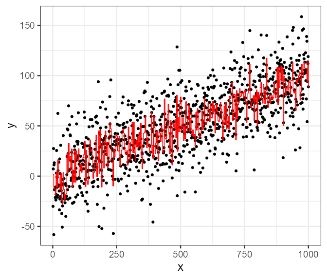
I illustrate that below (using R, but should be the same in python) by producing an incredibly overfit model for what is a simple linear regression (the only reason I didn't manage to put it through every single point exactly is the binning that LightGBM does, which produces 335 bins for the 1000 datapoints):

When I try this model on the test data, I get an unbiased estimate of the RMSE (sure, with a bit of uncertainty, but it's small enough for our purposes). What I get is 28.6. When I evaluate it in the way you propose, I get a RMSE of 20.6 (which is exactly the naïve estimate of the RMSE when evaluated directly on the training set), which is of course very overoptimistic for this model.

In fact, because we exactly know the data generating mechanism, we know that a linear regression is the optimal model and that (when trained on the training data and evaluated on the test data achieves 24.7 - sqrt(mean((test$y - predict(lm(y ~ x, data=train), newdata=test))^2))). I.e. the evaluation method claims a result that is better than anything that is even possible.

library(tidyverse)
library(lightgbm)

set.seed(1234)
train = tibble(x=1:1000, y=rnorm(n=1000, mean=x/10, sd=25))
test = tibble(x=seq(1,1000,0.1), y=rnorm(n=length(seq(1,1000,0.1)), mean=x/10, sd=25))

train %>%
  ggplot(aes(x=x, y=y)) +
  geom_point()

#### Train on training data 

lgb_train <- lgb.Dataset( data = as.matrix(train %>% dplyr::select(x)),
                         label = train$y)

lgb1 <- lightgbm(lgb_train, params=list(boosting="gbdt",
                                        objective="regression", 
                                        metric="rmse",
                                        num_iterations=1, 
                                        learning_rate=1.0, 
                                        max_bin=10000,
                                        max_depth=-1,
                                        num_leaves=10000,
                                        bagging_freq=0,
                                        min_data_in_leaf=1
                                        ))

##### Look at what it does

tibble( y = train$y,
        x = train$x,
        ypred = predict(lgb1, as.matrix(train %>% dplyr::select(x)))) %>%
  ggplot(aes(x=x,y=y)) +
  theme_bw(base_size=18) +
  geom_point() +
  geom_step(aes(y=ypred), col="red")

#### Sensible evaluation on test data:
test_predicted <- tibble(y = test$y,
                         predy = predict(lgb1, as.matrix(test %>% dplyr::select(x))))

test_predicted %>%
  summarize(metric = sqrt(mean(y-predy)^2))

##### Train on test data

lgb_train2 <- lgb.Dataset( data = as.matrix(test %>% dplyr::select(x)),
                           label = predict(lgb1, as.matrix(test %>% dplyr::select(x))))


lgb2 <- lightgbm(lgb_train2, params=list(boosting="gbdt",
                                        objective="regression", 
                                        metric="rmse",
                                        num_iterations=1, 
                                        learning_rate=1.0, 
                                        max_bin=10000,
                                        max_depth=-1,
                                        num_leaves=10000,
                                        bagging_freq=0,
                                        min_data_in_leaf=1))

##### Comparison to benchmark as before
train_predicted <- tibble(y = train$y,
                          predy = predict(lgb2, as.matrix(train %>% dplyr::select(x))))

train_predicted %>%
  summarize(metric = sqrt(mean(y-predy)^2))