Survival analysis with only censored event times?

Question

I have a dataset with destructive follow-up. That is, with a population starting at time 0, we are taking out a proportion at predetermined time points to see whether the event has occurred to them. The sampling is destructive, so we can't sample the same individuals repeatedly. In this case, we need to dissect a fish to determine whether the event has happened and we do this to a set number of fish at predetermined times. For example, we dissect 15 fish at 24h to know which animals have had the event, then we dissect another 15 animals at 48h and so on. I have done a logistic regression with time as one of the predictors and binary outcome (binomial family glm), but I wanted to ask if it's possible to use survival analysis for this type of data. I think what I have is left censored data for the animals where the event has occurred at time of dissection, and right censored for the animals where it hasn't occurred. In that case, there is only censored data, right? Is there a correct way of using this kind of data for survival analysis?

Edit: In this experiment, I have size of fish and temperature as covariates, so ideally, I would like to test whether these two variables affect the time to event. Both temperature and weight can be stratified ("small, medium, large" and "cold, medium, warm") as they are semi-controlled variables, but I'll probably get more information out of using the exact measurements rather than creating dummy variables. I can also add that the event is certain to happen eventually with the experiment designed to keep going until >95% of the fish are expected to have had the event. I also know for certain that none of the fish had the event at time 0. This then also would suggest that I have reasonable priors, so could take a bayesian approach.

Answer 1

It's not that you don't have events, it's just that you don't have exact times for the events. You do, however, have a lower and an upper limit to the time to each event. That's what's called "interval censored" data in general. In your situation, there's only 1 observation time per individual, so you have "current status" data as @Ben said in a comment. As you note, you have left-censored event times for cases with events (lower limit of 0) and right-censored event times for cases without events (upper limit of +Infinity).

Some types of survival analysis with such data are relatively straightforward. Let's take the reproducible data set provided in the answer from @AdamO (+1) and reformat it. Specify "L" and "R" as the left and right limits of the interval. It turns out that setting the lower (left) limit for left-censored event times to -Inf instead of 0 helps with some functions.

set.seed(123)
n <- 100
x <- rexp(n, 1/50)
t <- 10*(1+1:n%/% 10.1) ## assigned sacrifice timepoint
dissectData <- data.frame(dissectTime=t,event=x<t)
dissectData[,"L"] <- -Inf
dissectData[,"R"] <- Inf
dissectData[dissectData$event==FALSE,"L"] <- dissectData[dissectData$event==FALSE,"dissectTime"]
dissectData[dissectData$event==TRUE,"R"] <- dissectData[dissectData$event==TRUE,"dissectTime"]

That puts data into a form used by the "interval2" type of Surv object in the R survival package. That allows for simple descriptive survfit() processing (for 1 or more groups) and for parametric survival modeling. For example:

library(survival) 
plot(survfit(Surv(L, R, type="interval2") ~ 1, data = dissectData), bty="n",xlab="Time",ylab="Fraction Surviving")
curve(exp(-x/50),from=0,to=100,add=TRUE,col="red")

shows the estimated survival curve and its 95% confidence intervals (in black) along with the original continuous function used to generate the data sample (in red).

You can fit a parametric survival model this way, also. For example:

survreg(Surv(L, R, type="interval2") ~ 1, data = dissectData)

fits the default Weibull model to the data. With a more complicated data set including treatment groups and other outcome-associated covariates, you can specify (functions of) those as predictors instead of the simple ~1 intercept-only predictor used here for a single group. There are several other choices for survival distributions available, too.

You can't, however, fit a semi-parametric model like a Cox survival model via the survival package. For that you need specialized tools like those in the R icenReg package. That package works directly with "interval2" data. It also provides for Bayesian models like those recommended by @Björn in another answer (+1).

Your small set of known, fixed time points does recommend a binomial regression approach, but you didn't provide enough details to know if your model correctly takes the left censoring into account. A simple binomial model of fractions of animals with tumors over time is a model of tumor prevalence. That's OK for some purposes, and it can form the basis for tests of treatment effects with covariate adjustment. Prevalence data, however, leads to problems in interpretation in terms of tumor onset if the observed prevalence decreases at a later time period.

The answer from @AdamO provides a good way to deal with that problem, in a way that forces the cumulative hazard to be non-decreasing. Tutz and Schmid discuss ways to handle interval censoring in a binomial regression context in Section 3.7, "Subject-Specific Interval Censoring," of their Modeling Discrete Time-to-Event Data book.

Answer 2

This is a case of right censoring and (if there had been events) interval censoring. I.e. when a fish is event free when dissected, the event time is right censored (assuming all fish would eventually have the event). If you upon dissection a fish has the event, the event is interval censored to lie between time 0 and the time of dissection.

So far, so easy. One tricky bit is when you don't have any events, at all. E.g. simple maximum likelihood estimation based on asymptotics will break down here. However, firstly there's exact methods for some situations (e.g. if you assume the hazard rate to be constant over time) and secondly (more flexible and probably more usefully) there's Bayesian survival analysis. Going Bayesian here with informative (based on the best available prior information/what you elicit from experts) or weakly informative (wider than your prior assumptions suggest) prior distributions is very attractive.

Answer 3

Since the observation times are non-random, logistic regression can be used to estimate the event rate per each 24h interval. You can even just use proportions tests to estimate CIs, unless there are stratification features you want to implement, like species, weight, etc.

For fish sacrificed at time 1, denote the probability of event as $p_1$. At time 2, the event occurrence has probability $p_1 + p_2$. And so on. A standard survival analysis does not apply in this case because fish who were sacrificed at time 2 were not known to be event free at time 1, and so it would be inappropriate to include them in the denominator of "risk set" as non-events for the time 1 stratum as would be typical of a Cox model. This considerably simplifies the model, although knowing the event status for surviving fish at each time point would inform different models that could be considerably more powerful.

You can use these probabilities to report the cumulative incidence of the event. See R implementation to make things crystal clear.

set.seed(123)
n <- 100
x <- rexp(n, 1/50)
t <- 10*(1+1:n%/% 10.1) ## assigned sacrifice timepoint
p <- tapply(x < t, t, mean)
plot(unique(t), p, xlim=c(0, 100), ylim=c(0, 1), type='b')
segments(
  unique(t), 
  p-sqrt(p*(1-p)/10), 
  unique(t), 
  p+sqrt(p*(1-p)/10)
)

curve(pexp(x, 1/50), add=T, lty=2)

From this basic approach there are a number of interesting and more sophisticated things to consider.

• Is there a single-pass modeling procedure that constrains the empirical cumulative incidence to be strictly increasing? Consider maximum likelihood constraining $p_1 < (p_1+p_2) < \ldots $.

• Alternately, can a fitting procedure be used for the time-based event incidence to produce a stepwise increasing curve?

maximum likelihood approach

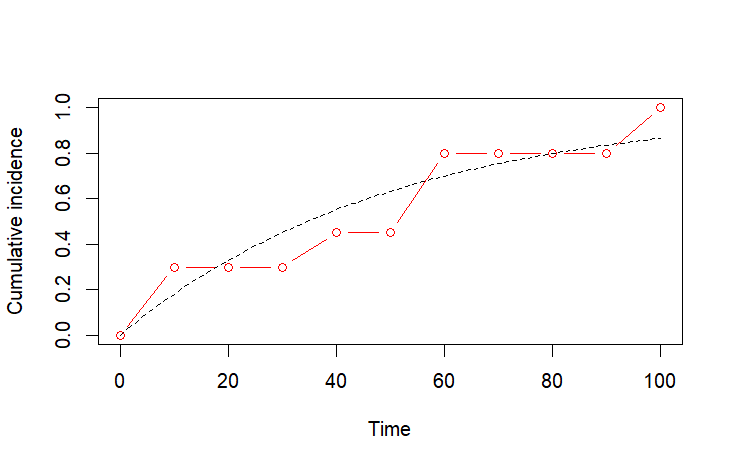
A convenient way to constrain the probability so that $p_2, p_3, \ldots >0 $ while keeping $p_1 + p_2 + \ldots < 1$ is to use the log odds. The result is somewhat better than the above approach.

## parameterize the log odds difference, constrain non-index LO to be positive, i.e. increasing probability
lodiff.to.p <- function(lodiff )  plogis(cumsum(c(lodiff[1], pmax(0, lodiff)[-1])))
negloglik <- function(lodiff) ## evaluate the joint likelihood
  -sum(dbinom(x=tapply(x<t, t, sum), size=table(t), prob=lodiff.to.p(lodiff), log=T))
mle <- nlm(negloglik, p=c(-3, rep(0.01, 9))) ## lucky guess
plot(c(0,unique(t)), c(0,lodiff.to.p(mle$estimate)), col='red', type='b', xlab='Time', ylab='Cumulative incidence')
curve(pexp(x, 1/50), add=T, lty=2)

curve fitting

We might use the empirical probability estimates to fit a monotonic increasing curve via least-squares. This approach is similar to the above, just swap binomial likelihood with normal.

negloglik <- function(mudiff) {
  mu <- pmin(1, cumsum(pmax(0, mudiff)))
  -sum(dnorm(x=p, mean = mu, sd=1, log=T))
}
mle <- nlm(negloglik, p=rep(0.1, 10))
mu <- pmin(1, cumsum(pmax(0, mle$estimate)))
plot(p, xlim=c(0, 10), ylim=c(0, 1), xlab='Time', ylab='Proportion with event')
lines(0:10, c(0,mu))