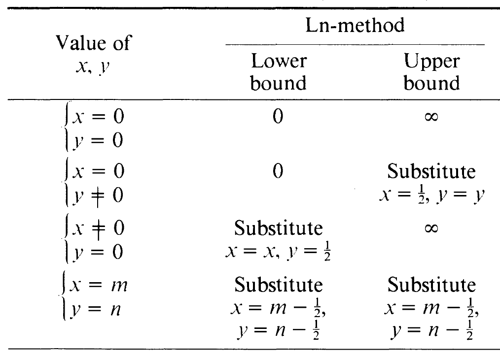
The paper by Koopman (1984) Confidence intervals for the ratio of two binomial proportions gives two methods for calculating the confidence interval. I am gonna explain the first one here as the confidence intervals can be calculated analytically (the second method uses an iterative procedure to find the confidence intervals numerically). First, consider the following 2x2 table:
                 Gold standard
               Positive Negative
Test positive     a        b
Test negative     c        d
The the likelihood ratio of a positive test is:
$$
LR_{+}=\frac{a/(a+c)}{b/(b+d)}
$$
and the likelihood ratio of a negative test is:
$$
LR_{-}=\frac{c/(a+c)}{d/(b+d)}
$$
These are basically the ratio of two proportions.
Confidence intervals using a normal approximation
Let $T = \frac{X/m}{Y/n}$, then the variable $\ln(T)$ isapproximately normally distributed with approximate mean $\ln(\theta)$ and estimated variance $\widehat{\sigma}^{2}=(1/x) - (1/m) + (1/y) - (1/n)$. An approximated two-sided $1-\alpha$ confidence interval for $\theta$ is given by:
$$
\{t\cdot \exp(-\xi_{1-\alpha/2}\cdot\hat{\sigma}), t\cdot \exp(\xi_{1-\alpha/2}\cdot\hat{\sigma})\}
$$
where $\xi_{1-\alpha/2}$ is the $1-\frac{1}{2}\alpha$ quantile of the standard normal distribution $\mathcal{N}(0,1)$ (for $\alpha = 0.05$ $\xi=1.96$) and $t$ is the observed value of $T$ (in your case, $t$ would be simply the observed likelihood ratios). In your case, $T$ is simply the likelihood ratios and $x=a, m=a+c, y=b, n=b+d$ for the positive LR or $x=c, m=a+c, y=d, n=b+d$ for the negative LR. Important: The paper also states procedures if $x=0, x=m, y=0$ or $y=n$:

If you have no false-positives ($b=y=0$ in the table above), then you can just substitute $b=1/2$ to calculate the lower bound of the confidence interval.
In this post, @whuber provides a similar approach: add $1/2$ to both $x$ and $y$ and add $1$ to both the $n$ and $m$. In this particular case, add $1/2$ to $a$ and $b$ and add $1$ to $(a+c)$ and $(b+d)$ for the positive LR and add $1/2$ to $c$ and $d$ and add $1$ to $(a+c)$ and $(b+d)$ for the negative LR.
Another formulation
The above confidence interval can be written differently:
$$
LR_{x}=\exp\left[\ln\left(\frac{p_1}{p_2}\right)\pm \xi_{1-\alpha/2}\cdot \sqrt{\frac{1-p_1}{p_{1}n_{1}}+\frac{1-p_2}{p_{2}n_{2}}} \right]
$$
where $\xi_{1-\alpha/2}$ is the $1-\frac{1}{2}\alpha$ quantile of the standard normal distribution. Note: For the positive LR, $p_1=\text{sensitivity}$ and $p_2=1-\text{specificity}$ and for the negative LR, $p_1=1-\text{sensitivity}$ and $p_2=\text{specificity}$ and $n_1 = a+c, n_2=b+d$.
Here is a little R function that carries out the calculations:
lr.ci <- function( m, sig.level=0.95 ) {

  alpha <- 1 - sig.level

  a <- m[1, 1]
  b <- m[1, 2]
  c <- m[2, 1]
  d <- m[2, 2]

  spec <- d/(b+d)
  sens <- a/(a+c)

  lr.pos <- sens/(1 - spec)

  if ( a != 0 & b != 0 ) {

    sigma2 <- (1/a) - (1/(a+c)) + (1/b) - (1/(b+d))

    lower.pos <- lr.pos * exp(-qnorm(1-(alpha/2))*sqrt(sigma2))

    upper.pos <- lr.pos * exp(qnorm(1-(alpha/2))*sqrt(sigma2))


  } else if ( a == 0 & b == 0 ) {

    lower.pos <- 0
    upper.pos <- Inf

  } else if ( a == 0 & b != 0 ) {

    a.temp <- (1/2)

    spec.temp <- d/(b+d)
    sens.temp <- a.temp/(a+c)

    lr.pos.temp <- sens.temp/(1 - spec.temp)

    lower.pos <- 0

    sigma2 <- (1/a.temp) - (1/(a.temp+c)) + (1/b) - (1/(b+d))

    upper.pos <- lr.pos.temp * exp(qnorm(1-(alpha/2))*sqrt(sigma2))

  } else if ( a != 0 & b == 0 ) {

    b.temp <- (1/2)

    spec.temp <- d/(b.temp+d)
    sens.temp <- a/(a+c)

    lr.pos.temp <- sens.temp/(1 - spec.temp)

    sigma2 <- (1/a) - (1/(a+c)) + (1/b.temp) - (1/(b.temp+d))

    lower.pos <- lr.pos.temp * exp(-qnorm(1-(alpha/2))*sqrt(sigma2))

    upper.pos <- Inf

  } else if ( (a == (a+c)) & (b == (b+d)) ) {

    a.temp <- a - (1/2)
    b.temp <- b - (1/2)

    spec.temp <- d/(b.temp+d)
    sens.temp <- a.temp/(a+c)

    lr.pos.temp <- sens.temp/(1 - spec.temp)

    sigma2 <- (1/a.temp) - (1/(a.temp+c)) + (1/b.temp) - (1/(b.temp+d))

    lower.pos <- lr.pos.temp * exp(-qnorm(1-(alpha/2))*sqrt(sigma2))

    upper.pos <- lr.pos.temp * exp(qnorm(1-(alpha/2))*sqrt(sigma2))

  }


  lr.neg <- (1 - sens)/spec

  if ( c != 0 & d != 0 ) {

    sigma2 <- (1/c) - (1/(a+c)) + (1/d) - (1/(b+d))

    lower.neg <- lr.neg * exp(-qnorm(1-(alpha/2))*sqrt(sigma2))

    upper.neg <- lr.neg * exp(qnorm(1-(alpha/2))*sqrt(sigma2))

  } else if ( c == 0 & d == 0 ) {

    lower.neg<- 0
    upper.neg <- Inf

  } else if ( c == 0 & d != 0 ) {

    c.temp <- (1/2)

    spec.temp <- d/(b+d)
    sens.temp <- a/(a+c.temp)

    lr.neg.temp <- (1 - sens.temp)/spec.temp

    lower.neg <- 0

    sigma2 <- (1/c.temp) - (1/(a+c)) + (1/d) - (1/(b+d))

    upper.neg <- lr.neg.temp * exp(qnorm(1-(alpha/2))*sqrt(sigma2))

  } else if ( c != 0 & d == 0 ) {

    d.temp <- (1/2)

    spec.temp <- d.temp/(b+d)
    sens.temp <- a/(a+c)

    lr.neg.temp <- (1 - sens.temp)/spec.temp

    sigma2 <- (1/c) - (1/(a+c)) + (1/d.temp) - (1/(b+d))

    lower.neg <- lr.neg.temp * exp(-qnorm(1-(alpha/2))*sqrt(sigma2))

    upper.neg <- Inf

  } else if ( (c == (a+c)) & (d == (b+d)) ) {

    c.temp <- c - (1/2)
    d.temp <- d - (1/2)

    spec.temp <- d.temp/(b+d)
    sens.temp <- a/(a+c.temp)

    lr.neg.temp <- (1 - sens.temp)/spec.temp

    sigma2 <- (1/c.temp) - (1/(a+c)) + (1/d.temp) - (1/(b+d))

    lower.neg <- lr.neg.temp * exp(-qnorm(1-(alpha/2))*sqrt(sigma2))

    upper.neg <- lr.neg.temp * exp(qnorm(1-(alpha/2))*sqrt(sigma2))

  }

  list(
    lr.pos=lr.pos, lower.pos=lower.pos, upper.pos=upper.pos,
    lr.neg=lr.neg, lower.neg=lower.neg, upper.neg=upper.neg
    )

}

