How to interpret peaks in probability density function?

Question

If a probability density function (created using kernel density estimation) exhibits peaks (not necessarily the mode), can we infer the presence of clusters or subgroups in the data?

Answer 1

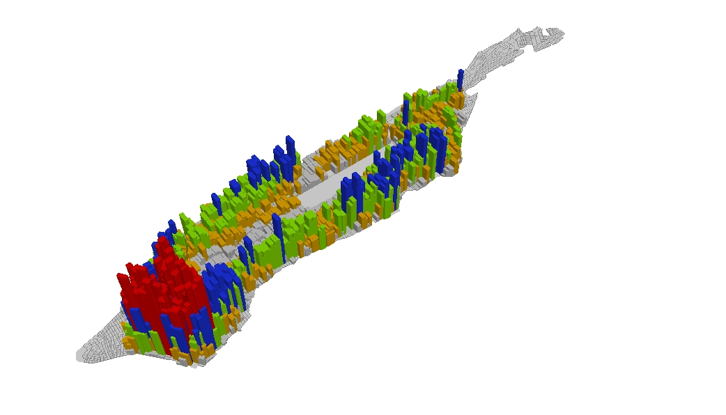
It depends on how you define or measure a peak. A local maximum of the KDE pdf could be the result of noise or represent one of many possible epicenters of a cluster. See the following population density map of Manhattan in 1990, where downtown Manhattan probably represents a single cluster, but contains multiple competing peaks.

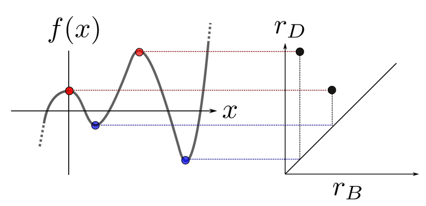
Now, call this a hammer in search of a nail, but as an applied topologist I would say that topology can be used to define the extent to which a peak is responsible/participates in a unique subgroup or cluster. Persistent homology analyzes the various peaks (maxima and minima) and measures the extent to which they represent a unique topological feature, vs. are part of a larger feature (vast oversimplification here). This works in all dimensions, but here is a visualization of persistence in 1D: the right-hand side shows the derived features, whose coordinates are the birth and death scales of each feature. The point further from the diagonal represents the big isolated peak corresponding, potentially, to a robust subgroup.

Another way of understanding persistence, and this can be made precise, is that the persistence of a topological feature, like an apparent cluster, captures the minimum amount of flattening needed to erase it.

Persistent homology, and applied topology more generally, has been applied extensively to clustering (at least in the literature), and provides, from my point of view, a very natural way of determining whether or not a peak corresponds to a real subgroup or something more transient.

Answer 2

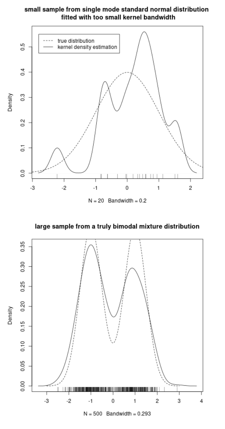
There are two ways to get peaks

1. If you are using kernel density estimation, then peaks may arrise as artifacts of the method. Especially when the kernel bandwidth is small and sample size is small.
2. The original distribution has truly peaks.

Example in R code

set.seed(1)

x = seq(-3,3,0.01)

y = rnorm(20,0,1)
plot(density(y, bw=0.2), main = "small sample from single mode standard normal distribution \n fitted with too small kernel bandwidth")
graphics::rug(y)

lines(x,dnorm(x), lty = 2)

legend(-2.8,0.55,c("true distribution", "kernel density estimation"), lty = c(2,1))

n = 500
y = rnorm(n,rbinom(n,1,0.5)*2-1,0.5)
plot(density(y), main = "large sample from a truly bimodal mixture distribution")
graphics::rug(y)

lines(x,(dnorm(x,1,0.5)+dnorm (x,-1,0.5))/2, lty = 2)

If the peaks in the estimated density have similar bandwidths as the kernel bandwidths, then it is difficult to differentiate between the two situations, and you should gather more data in order to figure out whether the peaks are artifacts or truly reflect the distribution of the population.

Answer 3

There are a variety of clustering methods based on probability density estimation. Most famous among density-based clustering methods are DBSCAN (and HDBSCAN), which connect points within certain distance thresholds. There are also level-set clustering methods (such as DeBaCL) which estimate a tree of clusters based on varying the threshold $t$ for level set $L_t := \{x: \hat{p}(x) > t \}$. Furthermore, there are mode-based clustering methods (such as the mean-shift algorithm) which identify modes and use these to define clusters, partitioning the space into regions where the gradients of the KDE density lead to each given mode. The mean-shift algorithm, interestingly, can be used to identify not only modes, but also ridges, which is useful for identifying cosmic filaments from astronomical data.

In fact, while mixture model clustering methods (eg KMeans, Gaussian Mixture Models) are more popular, density-based clustering methods are arguably statistically superior. Mixture models typically suffer from non-identifiability, and the distribution of the maximum-likelihood estimator is often hard to analyze. Meanwhile, the kernel density estimator has excellent and well-established statistical properties, so clustering methods based on it often carry stronger statistical guarantees. See Ryan Tibshirani's lecture notes on clustering for more on this topic: https://www.stat.cmu.edu/~ryantibs/statml/lectures/clustering.pdf.