Neural network training: Early stopping vs. reducing the number of neurons/layers

Question

Assuming we have a regression task (1D-output, values between 0.0 and 1.0) with 100 input dimensions and a classical MLP with one hidden layer.

When given 10000 training examples, a network with, for example, 50 neurons in the hidden layer has around 5000 trainable parameters and might overfit.

To avoid this, two (out of many) options are:

• apply early stopping (quit training when the validation loss no longer improves)
• reduce the model complexity (for example, only use 8 neurons in the hidden layer, thus having only around 800 trainable parameters).

Assuming training duration and model size are irrelevant, is there a consensus about which method of these two is to be preferred?

Does one method usually produce better results than the other?

Answer 1

Of course this decision is a difficult one without having a good understanding of the data, difficulty of the problem, and also the network architechture characteristics (e.g., activation functions) that you are considering. But as a rule of thumb (which might be very bad), you can make a decision about this based the following heuristic.

Perform your early stopping and measure:

• Your Training set error rate
• Your Development set error rate (do not touch your test set! reason).

Consider the following steps in order of appearance:

1. If your Training error is high, then you stopped too early. Let it continue for a while.

2. If the Training error stays high after you continued training, you actually have a high bias. Increase the complexity of your network.

3. If your Training error is okay and now is close to optimal/bayes (compared to Development error which is still relatively high at the current epoch), it means that your network had enough complexity to reach the "optimum" point but it had too much complexity, as your Development set has not reached that "optimal" point yet. This indicates that you need to reduce the complexity of your network (i.e., reduce #nodes).

4. If the alternative is true (i.e., Training error ~= Development error at the current epoch), then you are doing fine with complexity, so keep training your model with further epochs.

Note that you are making this decision at a certain epoch. Former or later epochs may present you a different story.

Finally, a no-brainer approach (which could be safer in my opinion) is that you can simply re-run the model training and follow each path (i.e., reducing #node vs. increasing #epoch) and then compare the performances. I think Andrew NG. has a pretty good lecture on this.

Answer 2

As an addition to the answers already given, I conducted a small experiment using the MNIST dataset:

• train/val split: 60000/10000
• input dimensions: 784
• hidden layers: 1
• output neurons: 10

The number of neurons in the hidden layer is what I used to adjust the model complexity.

import matplotlib.pyplot as plt

import numpy as np
import tensorflow as tf
import tensorflow_datasets as tfds


def normalize_img(image, label):
    """Normalizes images: `uint8` -> `float32`."""
    return tf.cast(image, tf.float32) / 255., label


(ds_train, ds_test), ds_info = tfds.load(
    "mnist",
    split=["train", "test"],
    shuffle_files=True,
    as_supervised=True,
    with_info=True,
)

# 60000
ds_train = ds_train.map(normalize_img, num_parallel_calls=tf.data.AUTOTUNE)
ds_train = ds_train.cache()
ds_train = ds_train.shuffle(ds_info.splits["train"].num_examples)
ds_train = ds_train.batch(128)
ds_train = ds_train.prefetch(tf.data.AUTOTUNE)

# 10000
ds_test = ds_test.map(normalize_img, num_parallel_calls=tf.data.AUTOTUNE)
ds_test = ds_test.batch(128)
ds_test = ds_test.cache()
ds_test = ds_test.prefetch(tf.data.AUTOTUNE)

for hidden_layer in range(2, 21):
    # https://www.tensorflow.org/datasets/keras_example
    model = tf.keras.models.Sequential([
        tf.keras.layers.Flatten(input_shape=(28, 28)),
        tf.keras.layers.Dense(hidden_layer, activation='elu'),
        tf.keras.layers.Dense(10)
    ])
    model.compile(
        optimizer=tf.keras.optimizers.Adam(0.001),
        loss=tf.keras.losses.SparseCategoricalCrossentropy(from_logits=True),
        metrics=[tf.keras.metrics.SparseCategoricalAccuracy()],
    )
    model.summary()

    history = model.fit(ds_train, epochs=100, validation_data=ds_test)

    layers = [28 * 28, hidden_layer, 10]
    params = model.count_params()
    val_loss = history.history["val_loss"]
    min_val_loss = min(val_loss)
    min_val_loss_min_ep = np.argmin(val_loss)
    min_val_loss_max_ep = len(val_loss) - np.argmin(val_loss[::-1]) - 1

    fig = plt.figure()
    ax = fig.add_subplot(1, 1, 1)
    ax.plot(history.epoch, history.history["loss"], label="train")
    ax.plot(history.epoch, history.history["val_loss"], label="val")
    ax.set_title(f"{layers=}; {params=}; {min_val_loss=:8.6};\n{min_val_loss_min_ep=}; {min_val_loss_max_ep=}")
    ax.set_ylim([0, 1.2])
    plt.xlabel("epochs")
    plt.ylabel("loss")
    plt.legend(loc="upper center")
    plt.grid()
    fig.savefig(f"{hidden_layer:02d}.png")

Resulting learning curves: https://imgur.com/a/SskHmNC

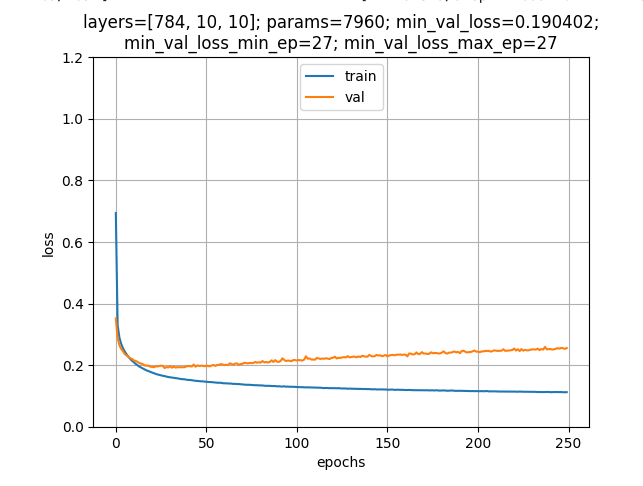
Example with 10 hidden neurons (does not need early stopping):

Example with 19 hidden neurons (does need early stopping around epoch 20):

Interpretation: From some number of neurons in the hidden layer upward, we need early stopping to get the best validation loss for these models. While I was somewhat cheering for the fewer-neurons solution to win, in this experiment, the solutions with more neurons (and early stopping!) performed better, i.e., the best validation loss was significantly lower.

Answer 3

EDIT:

A straight-forward answer from Yoshua Bengio

Page 11 in https://arxiv.org/abs/1206.5533

-> So use more neurons in combination with early stopping

I do not think these two things are equal.

Early stopping just stops you from overtraining, that is you train longer than necessary for a given set of hyperparameters, which results in a decreased validation loss. You can always use early stopping, independelty of the choice of hyperparameters.

However, reducing the number of neurons is an actual change to the architectures.

Early stopping can help you estimate the best possible validation loss for a given choice of architecture. So you can for example compare Model A to Model B. Early stopping helps you to identify the best loss, and hence the best parameters, for each model. And you now can adequately compare Model A to Model B. But in order find a well-performing model you need to change, hyperparameters that change the optimizer and or the architecture.

We can see also that when we train with 10 neurons as shown in OPs answer, we also get degradation of performance