7
$\begingroup$

When dealing with data $(X,Y)$ that is not time series data, for example $X=\text{weight}$ and $Y=\text{height}$, we can use OLS to estimate the coefficients $b_1$ and $b_0$ of a linear regression model $Y=b_1 X+b_0$ only if certain assumptions are met. One of the assumption is that the residuals are uncorrelated with each other. How do we check this assumption numerically? Do we simply perform the autocorrelation between the function $\text{res}(X)$ and it shifted version $\text{res}(X + \delta X)$?

The other assumption is that the $X$ values and the residuals $\text{res}(X)$ are uncorrelated. Do we simply do the sum of the pairwise products $X\cdot \text{res}(X)$ hoping that the sum is close to zero?

$\endgroup$

3 Answers 3

7
$\begingroup$

The second part of your question is already noted by Peter, which is fairly simple in implementation. I focus more on the first part of your question which can sometimes be more complex depending on the issue.

The easiest "test" of correlated errors is often just knowing what your correlational structures should be ahead of time. We should safely assume anything that can be partitioned into a group with shared characteristics will share some kind of correlational structure, each of which will have varying effects on the errors. Repeated measures and time series are the two most obvious types of data which will specifically have autocorrelation. How deeply correlated with the errors they are and how much that matters will vary, but modeling them directly certainly addresses much of this.

The typical way to check for autocorrelation is, as you say, some kind of autocorrelation function (ACF) plot or if needed a partial autocorrelation function (PACF) plot, shown below with clearly patterned residuals. A very simple simulated example of autocorrelated data and the ACF plot to detect it is written in R below, where the ACF plot shows an average autocorrelation of $.70$. The original source code is from here, but I annotate the code heavily to explain what its doing.

#### Set Seed ####
set.seed(123)

#### Simulate Autocorrelation ####
ar.epsilon <- arima.sim( # simulates time series
  list( # list to store info
    order = c(1,0,0), # simple AR(1) model with no differencing, etc.
    ar = 0.7 # level of autocorrelation
    ),
  n = 200, # number of observations
  sd=20 # fluctuation
  )

#### Simulate Data for Model ####
x <- rnorm(200) # normally distributed x
y = 50 + 25*x + ar.epsilon # intercept, slope, and autocorrelated residuals
df <- data.frame(x=x, y=y) # store data here

#### Fit Model ####
lm.mod <- lm(y ~ x, data=df) # fit model 

#### ACF Plot ####
acf(resid(lm.mod), # take residuals from model
    main = "ACF Plot of Residuals") # title
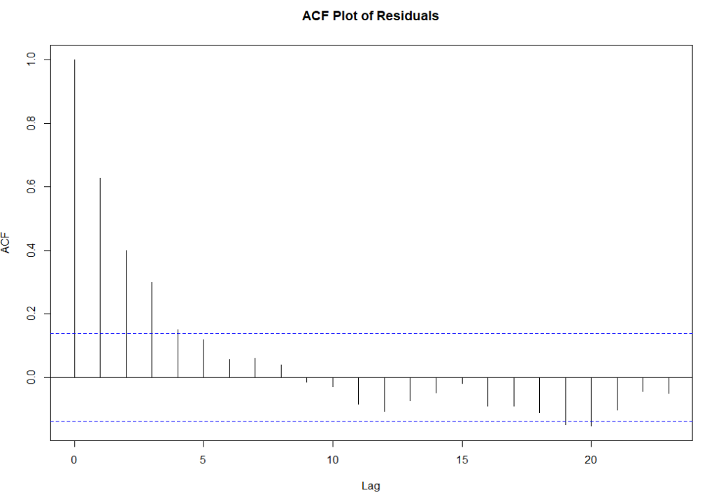
enter image description here

There also exist formal tests of autocorrelation like the Durbin-Watson or the Ljung-Box test, but I find such tests to be less useful than residual plots, and tests like these are known to have some problematic features. One important question you noted here:

Do we simply perform the autocorrelation between the function res($X$) and it shifted version res($X$ + $\delta X$) ?

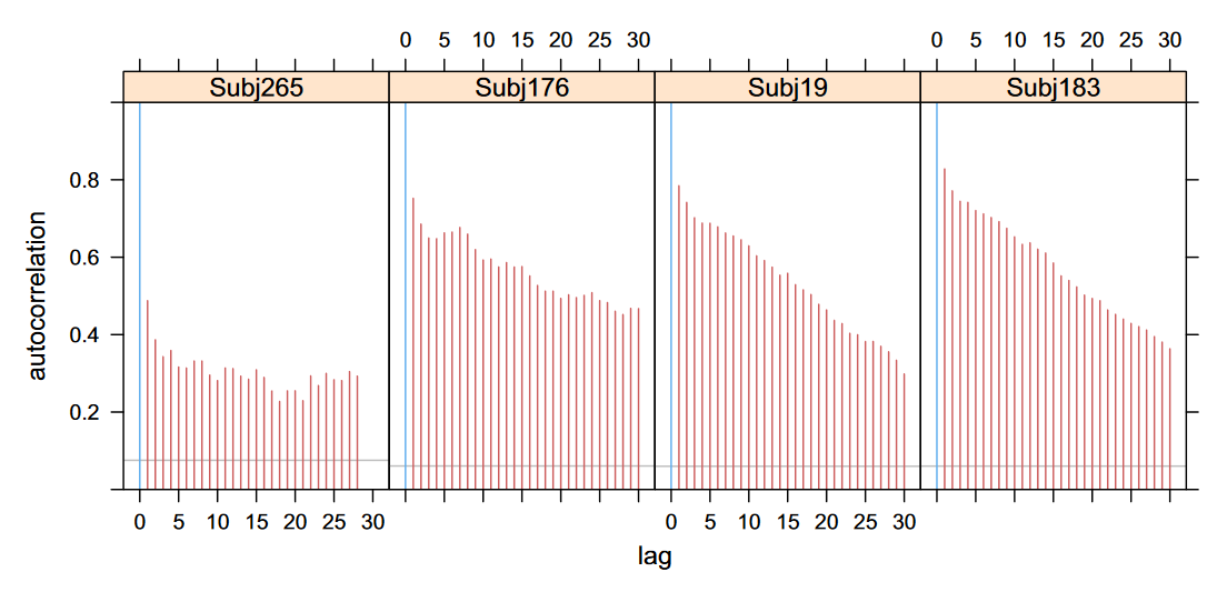
This will depend on the nature of your data. Often we can simply run the ACF or PACF plots on our residuals directly and examine away (one can adjust the amount of lag in these functions depending on the need). However, sometimes the residuals will have complex structural autocorrelation that is not easy to detect. Probably the easiest example of that is human trial data, where things like non-randomized trials can lead to people guessing more easily what the next trial will be and thus create correlated errors. Shown below are such trial autocorrelations, as explained in this article:
enter image description here

As shown, you would need to check by-subject ACF plots to determine if there are heavily correlated errors between trials which warrant concern, which one can program from the article above. Some implementations of time series in psychology may also be instructive of when these things pop up in human research which may not be "typical" time series.

$\endgroup$
3
  • 1
    $\begingroup$ +1 for the nice compilation. $\endgroup$ Commented Dec 28, 2023 at 1:06
  • $\begingroup$ +1 for a good summary of these methods. But ... would you do this for the situation outlined in the problem? I mean, it can't hurt (except in use of time) but if there is no reason to suspect autocorrelation, would you take the time? $\endgroup$
    – Peter Flom
    Commented Dec 28, 2023 at 10:02
  • $\begingroup$ Probably wouldnt bother, but figured I would illustrate when it would be useful to determine. Generally speaking you should probably already know if its going to be a problem before you end up checking, hence the bolded statement. $\endgroup$ Commented Dec 28, 2023 at 10:16
6
$\begingroup$

For the first assumption, with data that is not longitudinal and not clustered in some other way (e.g. by geography), I think it is just assumed. I don't recall ever seeing a test of this. Of course, there might be one, or my mind just be blanking it out.

For the second assumption, the usual way is graphically, with a plot of one vs. the other, and maybe a smoothed line added.

$\endgroup$
5
$\begingroup$

Adding to @Shawn Hemelstrand's already existing excellent answer, dependence/correlation cannot be diagnosed from data unless it is governed either by the order of observations or by known external variables (spatial location, group membership in grouped data). It can exist and cause trouble, but the data cannot tell us that this happens. See

Hennig, C. Parameters not empirically identifiable or distinguishable, including correlation between Gaussian observations. Stat Papers (2023). https://doi.org/10.1007/s00362-023-01414-3

(The paper mentions a further situation that allows for identification of dependence, but this is rather artificial and probably irrelevant in most practical settings.)

The bad news is that this means model assumptions may be critically violated in a way that we cannot see from the data. It is therefore of crucial importance to know the meaning of the data and to think hard of potential reasons for dependence other than the standard things to look for (i.e., temporal autocorrelation and repeated measures/grouped data). Even if these cannot be modelled, knowing about this means that we should be more careful avoiding overinterpretation of results.

A similar issue holds for potentially nonidentical distributions that play out in a nonstandard way (standard would be for example growing residual variance along an x-variable).

$\endgroup$
1
  • $\begingroup$ Thanks for the paper. That is an interesting read (+1). $\endgroup$ Commented Dec 29, 2023 at 2:19

Your Answer

By clicking “Post Your Answer”, you agree to our terms of service and acknowledge you have read our privacy policy.

Not the answer you're looking for? Browse other questions tagged or ask your own question.