2
$\begingroup$

I have two sample sets that consist of independent trials of a binomial variable X = {X0, X1}. For the remainder, I denote the probabilities as p0= p(X=X0) and p1= p(X=X1); the sample sizes as N1 and N2 and the binomial coefficients as C1 and C2.

1st Sample set: N1= 10 and the count of X0 observations is 2.

Hence, the maximum likelihood estimation (MLE) for p0=2/10. The likelihood function for this distribution is: Lik1 = C1 * (p0^2) * (1-p0)^8, which is plotted as:
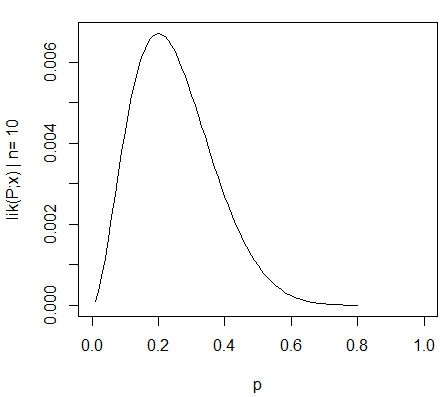
MLE of p0 for N1

2nd Sample set: N2= 100 and the count of X0 observations is 20.

Hence, the maximum likelihood estimation (MLE) for p0=20/100. The likelihood function for this distribution is: Lik2 = C2 * (p0^20) * (1-p0)^80, which is plotted as:
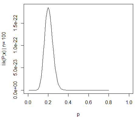
enter image description here

I know this much: As N is increased, lik(P;x) becomes more sharply peaked around the MLE (0.2), which means the width of the confidence interval decreases. I also understand that a confidence interval is not a probability statement for the MLE (0.2) since the MLE is a fixed value and not a random variable.

What I do not know: I am using an algorithm (i.e. Naive Bayes) that requires the multiplication of the MLEs of multiple variables similar to X. For instance: P(Class|X1,X2) = D * P(X1|Class)*P(X2|Class)*P(Class), where D is the normaliser and I estimate all P(Xn|Class)'s via MLE.

Is there a statistically valid method, whereby I can incorporate a confidence weight (derived from the sample size) for each independent variable's MLE? In other words, I want to be able to attach a sample-size-related confidence weight to each MLE while multiplying them. I hope the question is clear enough.

Reading around a bit, I found that the approximate standard error for the MLE can be calculated by 1/sqrt(-lik''(P;x)) where -lik''(P;x) is the second derivative of the likelihood function wrt p0 and is called the observed information. But I guess multiplying each MLE by its standard error does not make much sense..

$\endgroup$
4
  • 1
    $\begingroup$ My hunch is that you might be able to repeatedly apply Bayes theorem, starting with an uninformative Beta prior (see this answer for an example of a single application in the Beta/Binomial model). Then you would effectively be multiplying your MLEs together and incorporating the uncertainty directly. Would be interesting to know more about your algorithm to see if this is applicable. $\endgroup$
    – TooTone
    Commented Aug 16, 2013 at 14:49
  • $\begingroup$ Thank you, I updated my question (the 'What I do not know' bit) to explain the algorithm. The relevant part is: I just multiply the MLEs of some conditional probabilities of (assumedly) independent varibales. I am familiar with Bayesian learning, priors, likelihoods, etc. but could not envisage how repeatedly applying Bayes theorem would help. Can you elaborate in an answer? $\endgroup$
    – Zhubarb
    Commented Aug 16, 2013 at 15:46
  • $\begingroup$ thanks, stating the Naive Bayes explicitly makes the question clearer. I need to think some more about what I wrote earlier. I am pretty tired and not sure whether I got myself into a muddle or had a reasonable idea. Will have a think but will be away from my computer for a week or so... $\endgroup$
    – TooTone
    Commented Aug 16, 2013 at 22:47
  • $\begingroup$ My hunch about applying Bayes theorem was wrong, but it's still reasonable to think that you should somehow be able to "multiply the likelihoods". I've written an answer below where I take a sampling approach. $\endgroup$
    – TooTone
    Commented Aug 28, 2013 at 22:33

2 Answers 2

1
$\begingroup$

The most practical approach I have come up with is to sample from the likelihoods. I can't say that this is statistically valid, but it does seem to make sense intuitively and take account of the information that the likelihoods provide, giving narrower intervals where the likelihoods are narrower. The motivation behind what I've done is to perturb the inputs to understand the stability of an estimate. And the likelihoods give information about how much to perturb them.

A rough and ready implementation in R is as follows:

set.seed(99)

acc <- 1000
lik1 <- function(p) { p^2 * (1-p)^8 }
lik2 <- function(p) { p^20 * (1-p)^80 }
x <- (1:acc)/acc 
clik1 <- cumsum(lik1(x))
clik2 <- cumsum(lik2(x))

nrand <- 1000000
samplelik1 <- findInterval(runif(nrand, max=clik1[length(clik1)]), clik1) / acc
samplelik2 <- findInterval(runif(nrand, max=clik2[length(clik2)]), clik2) / acc
quantile(samplelik1*samplelik2, c(.025,.975))
    2.5%    97.5% 
    0.011319 0.114240

Here, I've normalized the likelihood and treated it as a pdf for the probability (which isn't valid for several reasons but might serve your purpose). So clik1 is the "cdf", and the probability integral transform is used in the standard way to go from a uniform random variable, using runif, to sample the desired random variable via the inverse cdf, using findInterval.

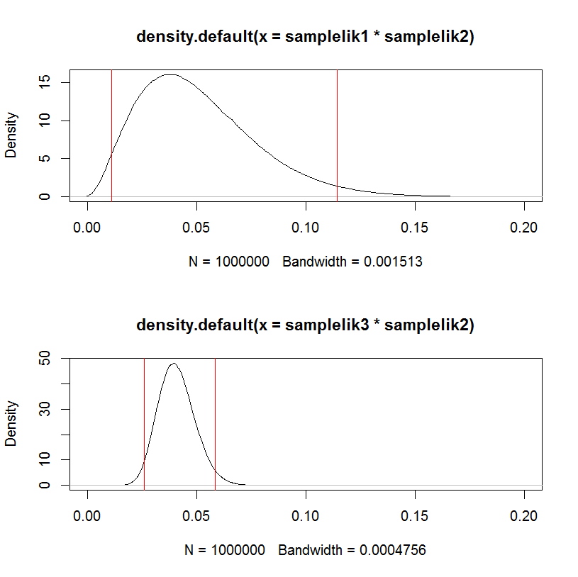
As a test, replacing the first likelihood samplelik1 with a narrower one samplelik3 gives a narrower interval.

lik3 <- function(p) { p^200 * (1-p)^800 }
clik3 <- cumsum(lik3(x))
samplelik3 <- findInterval(runif(nrand, max=clik3[length(clik3)]), clik3) / acc
quantile(samplelik3*samplelik2, c(.025,.975))
    2.5%      97.5% 
    0.02594400 0.05863703 

This can be visualized in a hacky way:

par(mfrow=c(2,1))
plot(density(samplelik1*samplelik2),xlim=c(0,0.2));
abline(v=quantile(samplelik1*samplelik2, c(.025,.975)), col="red")
plot(density(samplelik3*samplelik2),xlim=c(0,0.2));
abline(v=quantile(samplelik3*samplelik2, c(.025,.975)), col="red")

enter image description here

$\endgroup$
6
  • $\begingroup$ Thanks a lot. If I understand correctly: clik1 is the CDF of lik1. First, using runif(), you draw nrand samples between 0 and last element of clik2. Then you put these into findInterval() to get samplelik1. This is where I got lost. What is samplelik1 statistically? $\endgroup$
    – Zhubarb
    Commented Aug 29, 2013 at 15:43
  • $\begingroup$ @Berkan I think you've understood it well, and you are right to raise a statistical eyebrow (I wasn't comfortable after sleeping on it). I've added some more explanation. This approach certainly seems to work in the sense of providing an interval for the required probability which behaves in the expected way. However a theoretical justification is harder -- if you're comfortable viewing the normalized likelihoods as pdfs for your beliefs about p0 or p1 then there is some justification for taking the 0.025 and 0.975 boundaries as a confidence interval, but it's a big if. Hth, anyway. $\endgroup$
    – TooTone
    Commented Aug 29, 2013 at 16:50
  • $\begingroup$ I see, thanks. I am no stats expert but what you describe makes intuitive sense. I was looking at the code and did: plot(x,clik1) and plot(x,clik2). The latter converges to the max value of the y axis (since the confidence interval is tighter) a lot faster( at about 0.3, whereas for the former this is around 0.5). Do you think I can use this information to devise individual weights for lik1 and lik2? $\endgroup$
    – Zhubarb
    Commented Aug 30, 2013 at 8:12
  • 1
    $\begingroup$ It's intuitive but only really makes sense if you accept the normalized likelihood as a pdf -- I know enough stats to know there's a lot I don't know and others on CV are better qualified to judge than me. I don't think that plotting the cumulative function gives you much more than plotting the original. Not sure what you mean by "individual weights" but you might be looking for confidence intervals, in which case you can either get a confidence interval for a binomial parameter directly or derive it from the likelihood (example). $\endgroup$
    – TooTone
    Commented Aug 30, 2013 at 12:46
  • $\begingroup$ OK, thanks a lot for taking the time. I am not accepting the answer yet, in case someone else may come up with an alternative answer. $\endgroup$
    – Zhubarb
    Commented Aug 30, 2013 at 13:02
1
$\begingroup$

One branch of statistics that works on combining estimates, whereby each estimate can be measured with different levels of precision, is meta analysis. That might be a literature worth investigating. Often this boils down to computed an weighted sum of coefficients, whereby each coefficient receives a weight of $se^{-2}$, where $se$ is short for the standard error.

$\endgroup$
2
  • $\begingroup$ do you mean (std error)^-2? $\endgroup$
    – Zhubarb
    Commented Aug 16, 2013 at 14:40
  • $\begingroup$ good point, I eddited the answer to clarify what I mean with $se$. $\endgroup$ Commented Aug 16, 2013 at 15:28

Your Answer

By clicking “Post Your Answer”, you agree to our terms of service and acknowledge you have read our privacy policy.

Not the answer you're looking for? Browse other questions tagged or ask your own question.