11
$\begingroup$

It is clear the product of normal distributed variables is not normal distributed. For example, if $X \sim N( \mu_1,\sigma_1^2)$, $Y \sim N( \mu_2,\sigma_2^2)$, then $XY$ does not has the distribution of $ N( \mu_1 \mu_2,\mu_1^2 \sigma_1^2+\mu_2^2\sigma_1^2)$.

I have been told that even if the distribution of $XY$ is not normal distribution, the distribution of $XY$ is near to normal distribution, when $\mu_1$ and $\mu_2$ are not so small, $\sigma_1$ and $\sigma_2$ are not so big. Is it true?

Try following R code:

    n1 <- rnorm(10000,0,.005)
    n2 <- rnorm(10000,0,.005)
    n  <- n1*n2
    d  <- density(n)
    plot(d,lwd=2)
    x  <- par('usr')
    dn <- dnorm(d$x,mean=mean(n),sd=sd(n))
    x  <- seq(x[1],x[2],length.out=length(dn))
    lines(x, dn ,col=2, lwd=2)
    legend('topright', legend=c('Estimated density', 'Normal 
    distribution'), lwd=2, lty=c(1,1),col=c(1,2))
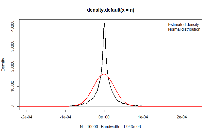
Density estimation when <span class=$\sigma_1=\sigma_2=0.005$" />

It seems only when two conditions are both meet, the distribution is near normal. Is there any theoretical analysis?

$\endgroup$
6
  • 1
    $\begingroup$ Do you intend that X and Y be independent? Your variance term looks wrong. If they're more generally dependent, it looks even more wrong. But yes, Yes, if the coefficients of variation are small, the product of two independent normals is fairly normal. $\endgroup$
    – Glen_b
    Commented Sep 4, 2013 at 2:27
  • $\begingroup$ Yes, they are independent. $\endgroup$
    – Kattern
    Commented Sep 6, 2013 at 6:49
  • 1
    $\begingroup$ I have updated some R code in the question. As seen in the figure, even if the coefficients of variation are small, the final distribution still not near normal. It seems there are more restrictions. $\endgroup$
    – Kattern
    Commented Sep 6, 2013 at 7:11
  • $\begingroup$ Please check the definition of coefficient of variation carefully, and try again with small coefficient of variation (yours aren't small!) $\endgroup$
    – Glen_b
    Commented Sep 6, 2013 at 7:28
  • 6
    $\begingroup$ Since $XY=(X/2+Y/2)^2 - (X/2-Y/2)^2$ and $X/2+Y/2\sim N(\mu_1/2+\mu_2/2,\sigma_1^2/4+\sigma_1^2/4)$ and $X/2-Y/2\sim N(\mu_1/2-\mu_2/2,\sigma_1^2/4+\sigma_1^2/4)$, it follows that $XY$ is a multiple of the difference of two non-central $\chi^2$ distributions, each with one degree of freedom. (They will be correlated when $\sigma_1\ne\sigma_2$, but that's not going to change the tail behavior of the difference unless one of the $\sigma_i$ dominates the other). That makes it apparent that $XY$ usually won't look at all Normal and provides a good source of counterexamples. $\endgroup$
    – whuber
    Commented Sep 6, 2013 at 16:01

1 Answer 1

7
$\begingroup$

(this answer uses parts of @whuber's comment)

Let $X,Y$ be two independent normals. We can write the product as $$ XY = \frac14 \left( (X+Y)^2 - (X-Y)^2 \right) $$ will have the distribution of the difference (scaled) of two noncentral chisquare random variables (central if both have zero means). Note that if the variances are equal, the two terms will be independent. Since chisquare distribution is a case of gamma, Generic sum of Gamma random variables is relevant. I will give a very special case of this, taken from the encyclopedic reference https://www.amazon.com/Probability-Distributions-Involving-Gaussian-Variables/dp/0387346570

When $X$ and $Y$ are independent, zero-mean with possibly different variances the density function of the product $Z=XY$ is given by $$ f(z)= \frac1{\pi \sigma_1 \sigma_2} K_0(\frac{|z|}{\sigma_1 \sigma_2}) $$ where $K_0$ is the modified Bessel function of the second kind.

This can be written in R as

    dprodnorm  <-  function(x, sigma1=1, sigma2=1) {
       (1/(pi*sigma1*sigma2)) * besselK(abs(x)/(sigma1*sigma2),  0)
    }
    ### Numerical check:
    integrate( function(x) dprodnorm(x), lower=-Inf,  upper=Inf)
    0.9999999 with absolute error < 3e-06

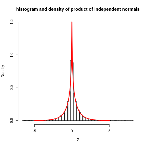
Let us plot this, together with some simulations:

    set.seed(7*11*13)  
    Z  <-  rnorm(10000) * rnorm(10000)
    
    hist(Z, prob=TRUE, nclass="scott", ylim=c(0, 1.5), 
            main="histogram and density of product of independent 
                  normals")
    plot( function(x) dprodnorm(x),  from=-5,  to=5,  n=1001,  
          col="red", add=TRUE, lwd=3)
    ### Change to nclass="fd" gives a closer fit

histogram and density of product of two independent normals

The plot shows quite clearly that the distribution is not close to normal.

The stated reference do also give more involved cases (non-zero means ...) but then expressions for density functions becomes so complicated that they only gives characteristic function, which still are reasonably simple, and can be inverted to get densities.

$\endgroup$

Your Answer

By clicking “Post Your Answer”, you agree to our terms of service and acknowledge you have read our privacy policy.

Not the answer you're looking for? Browse other questions tagged or ask your own question.