You wouldn't normally call the observed value an 'estimated value'.
However, in spite of that, the observed value is nevertheless technically an estimate of the mean at its particular $x$, and treating it as an estimate will actually tell us the sense in which OLS is better at estimating the mean there.
Generally speaking regression is used in the situation where if you were to take another sample with the same $x$'s, you would not get the same values for the $y$'s. In ordinary regression, we treat the $x_i$ as fixed/known quantities and the responses, the $Y_i$ as random variables (with observed values denoted by $y_i$).
Using a more common notation, we write
$$Y_i = \alpha + \beta x_i + \varepsilon_i$$
The noise term, $\varepsilon_i$, is important because the observations don't lie right on the population line (if they did there'd be no need for regression; any two points would give you the population line); the model for $Y$ must account for the values it takes, and in this case, the distribution of the random error accounts for the deviations from the ('true') line.
The estimate of the mean at point $x_i$ for ordinary linear regression has variance
$$\Big(\frac{1}{n} + \frac{(x_i-\bar{x})^2}{\sum(x_i-\bar{x})^2}\Big)\,\sigma^2$$
while the estimate based on the observed value has variance $\sigma^2$.
It's possible to show that for $n$ at least 3, $\,\frac{1}{n} + \frac{(x_i-\bar{x})^2}{\sum(x_i-\bar{x})^2}$ is no more than 1 (but it may be - and in practice usually is - much smaller). [Further, when you estimate the fit at $x_i$ by $y_i$ you're also left with the issue of how to estimate $\sigma$.]
But rather than pursue the formal demonstration, ponder an example, which I hope might be more motivating.
Let $v_f = \frac{1}{n} + \frac{(x_i-\bar{x})^2}{\sum(x_i-\bar{x})^2}$, the factor by which the observation variance is multiplied to get the variance of the fit at $x_i$.
However, let's work on the scale of relative standard error rather than relative variance (that is, let's look at the square root of this quantity); confidence intervals for the mean at a particular $x_i$ will be a multiple of $\sqrt{v_f}$.
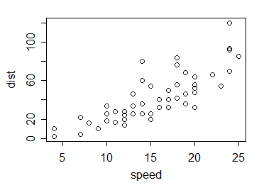
So to the example. Let's take the cars data in R; this is 50 observations collected in the 1920s on the speed of cars and the distances taken to stop:

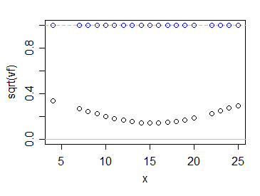
So how do the values of $\sqrt{v_f}$ compare with 1? Like so:

The blue circles show the multiples of $\sigma$ for your estimate, while the black ones show it for the usual least squares estimate. As you see, using the information from all the data makes our uncertainty about where the population mean lies substantially smaller - at least in this case, and of course given that the linear model is correct.
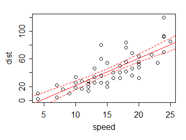
As a result, if we plot (say) a 95% confidence interval for the mean for each value $x$ (including at places other than an observation), the limits of the interval at the various $x$'s are typically small compared to the variation in the data:

This is the benefit of 'borrowing' information from data values other than the present one.
Indeed, we can use the information from other values - via the linear relationship - to get good estimates the value at places where we don't even have data. Consider that there's no data in our example at x=5, 6 or 21. With the suggested estimator, we have no information there - but with the regression line we can not only estimate the mean at those points (and at 5.5 and 12.8 and so on), we can give an interval for it -- though, again, one that relies on the suitability of the assumptions of linearity (and constant variance of the $Y$s, and independence).

