There are a number of options available when dealing with heteroscedastic data. Unfortunately, none of them is guaranteed to always work. Here are some options I'm familiar with:
- transformations
- Welch ANOVA
- weighted least squares
- robust regression
- heteroscedasticity consistent standard errors
- bootstrap
- Kruskal-Wallis test
- ordinal logistic regression
Update: Here is a demonstration in R of some ways of fitting a linear model (i.e., an ANOVA or a regression) when you have heteroscedasticity / heterogeneity of variance.
Let's start by taking a look at your data. For convenience, I have them loaded into two data frames called my.data (which is structured like above with one column per group) and stacked.data (which has two columns: values with the numbers and ind with the group indicator).
We can formally test for heteroscedasticity with Levene's test:
library(car)
leveneTest(values~ind, stacked.data)
# Levene's Test for Homogeneity of Variance (center = median)
#       Df F value   Pr(>F)
# group  2  8.1269 0.001153 **
#       38
Sure enough, you have heteroscedasticity. We'll check to see what the variances of the groups are. A rule of thumb is that linear models are fairly robust to heterogeneity of variance so long as the maximum variance is no more than $4\!\times$ greater than the minimum variance, so we'll find that ratio as well:
apply(my.data, 2, function(x){ var(x, na.rm=T) })
#          A          B          C
# 0.01734578 0.33182844 0.06673060
var(my.data$B, na.rm=T) / var(my.data$A, na.rm=T)
# [1] 19.13021
Your variances differ substantially, with the largest, B, being $19\!\times$ the smallest, A. This is a problematic level of heteroscedsaticity.
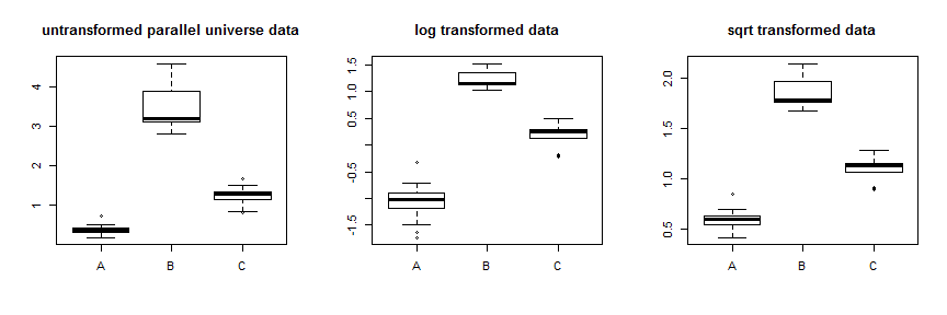
You had thought to use transformations such as the log or square root to stabilize the variance. That will work in some cases, but Box-Cox type transformations stabilize variance by squeezing the data asymmetrically, either squeezing them downwards with the highest data squeezed the most, or squeezing them upwards with the lowest data squeezed the most. Thus, you need the variance of your data to change with the mean for this to work optimally. Your data have a huge difference in variance, but a relatively small difference amongst the means and medians, i.e., the distributions mostly overlap. As a teaching exercise, we can create some parallel.universe.data by adding $2.7$ to all B values and $.7$ to C's to show how it would work:
parallel.universe.data = with(my.data, data.frame(A=A, B=B+2.7, C=C+.7))
apply(parallel.universe.data,       2, function(x){ var(x, na.rm=T) })
#          A          B          C
# 0.01734578 0.33182844 0.06673060
apply(log(parallel.universe.data),  2, function(x){ var(x, na.rm=T) })
#          A          B          C
# 0.12750634 0.02631383 0.05240742
apply(sqrt(parallel.universe.data), 2, function(x){ var(x, na.rm=T) })
#          A          B          C
# 0.01120956 0.02325107 0.01461479
var(sqrt(parallel.universe.data$B), na.rm=T) /
var(sqrt(parallel.universe.data$A), na.rm=T)
# [1] 2.074217
Using the square root transformation stabilizes those data quite well. You can see the improvement for the parallel universe data here:

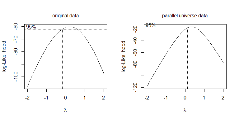
Rather than just trying different transformations, a more systematic approach is to optimize the Box-Cox parameter $\lambda$ (although it is usually recommended to round that to the nearest interpretable transformation). In your case either the square root, $\lambda = .5$, or the log, $\lambda = 0$, are acceptable, though neither actually works. For the parallel universe data, the square root is best:
boxcox(values~ind, data=stacked.data,    na.action=na.omit)
boxcox(values~ind, data=stacked.pu.data, na.action=na.omit)

Since this case is an ANOVA (i.e., no continuous variables), one way to deal with heterogeneity is to use the Welch correction to the denominator degrees of freedom in the $F$-test (n.b., df = 19.445, a fractional value, rather than df = 38):
oneway.test(values~ind, data=stacked.data, na.action=na.omit, var.equal=FALSE)
#  One-way analysis of means (not assuming equal variances)
#
# data:  values and ind
# F = 4.1769, num df = 2.000, denom df = 19.445, p-value = 0.03097
A more general approach is to use weighted least squares. Since some groups (B) spread out more, the data in those groups provide less information about the location of the mean than the data in other groups. We can let the model incorporate this by providing a weight with each data point. A common system is to use the reciprocal of the group variance as the weight:
wl = 1 / apply(my.data, 2, function(x){ var(x, na.rm=T) })
stacked.data$w = with(stacked.data, ifelse(ind=="A", wl[1],
                                           ifelse(ind=="B", wl[2], wl[3])))
w.mod = lm(values~ind, stacked.data, na.action=na.omit, weights=w)
anova(w.mod)
# Response: values
#           Df Sum Sq Mean Sq F value  Pr(>F)
# ind        2   8.64  4.3201  4.3201 0.02039 *
# Residuals 38  38.00  1.0000
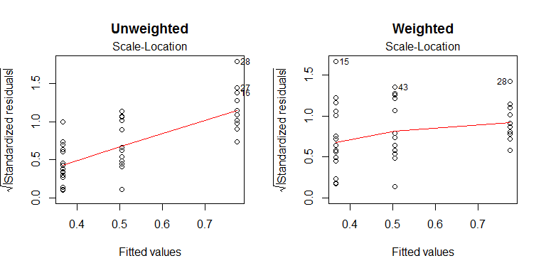
This yields slightly different $F$ and $p$-values than the unweighted ANOVA (4.5089, 0.01749), but it has addressed the heterogeneity well:

Weighted least squares is not a panacea, however. One uncomfortable fact is that it is only just right if the weights are just right, meaning, among other things, that they are known a-priori. It does not address non-normality (such as skew) or outliers, either. Using weights estimated from your data will often work fine, though, particularly if you have enough data to estimate the variance with reasonable precision (this is analogous to the idea of using a $z$-table instead of a $t$-table when you have $50$ or $100$ degrees of freedom), your data are sufficiently normal, and you don't appear to have any outliers. Unfortunately, you have relatively few data (13 or 15 per group), some skew and possibly some outliers. I'm not sure that these are bad enough to make a big deal out of, but you could mix weighted least squares with robust methods. Instead of using the variance as your measure of spread (which is sensitive to outliers, especially with low $N$), you could use the reciprocal of the inter-quartile range (which is unaffected by up to 50% outliers in each group). These weights could then be combined with robust regression using a different loss function like Tukey's bisquare:
1 / apply(my.data,       2, function(x){ var(x, na.rm=T) })
#         A         B         C
# 57.650907  3.013606 14.985628
1 / apply(my.data,       2, function(x){ IQR(x, na.rm=T) })
#        A        B        C
# 9.661836 1.291990 4.878049

rw = 1 / apply(my.data, 2, function(x){ IQR(x, na.rm=T) })
stacked.data$rw = with(stacked.data, ifelse(ind=="A", rw[1],
                                            ifelse(ind=="B", rw[2], rw[3])))
library(robustbase)
w.r.mod = lmrob(values~ind, stacked.data, na.action=na.omit, weights=rw)
anova(w.r.mod, lmrob(values~1,stacked.data,na.action=na.omit,weights=rw), test="Wald")
# Robust Wald Test Table
#
# Model 1: values ~ ind
# Model 2: values ~ 1
# Largest model fitted by lmrob(), i.e. SM
#
#   pseudoDf Test.Stat Df Pr(>chisq)
# 1       38
# 2       40    6.6016  2    0.03685 *
The weights here aren't as extreme. The predicted group means differ slightly (A: WLS 0.36673, robust 0.35722; B: WLS 0.77646, robust 0.70433; C: WLS 0.50554, robust 0.51845), with the means of B and C being less pulled by extreme values.
In econometrics the Huber-White ("sandwich") standard error is very popular. Like the Welch correction, this does not require you to know the variances a-priori and doesn't require you to estimate weights from your data and/or contingent on a model that may not be correct. On the other hand, I don't know how to incorporate this with an ANOVA, meaning that you only get them for the tests of individual dummy codes, which strikes me as less helpful in this case, but I'll demonstrate them anyway:
library(sandwich)
mod = lm(values~ind, stacked.data, na.action=na.omit)
sqrt(diag(vcovHC(mod)))
# (Intercept)        indB        indC
#  0.03519921  0.16997457  0.08246131
2*(1-pt(coef(mod) / sqrt(diag(vcovHC(mod))), df=38))
#  (Intercept)         indB         indC
# 1.078249e-12 2.087484e-02 1.005212e-01
The function vcovHC calculates a heteroscedasticicy consistent variance-covariance matrix for your betas (your dummy codes), which is what the letters in the function call stand for. To get standard errors, you extract the main diagonal and take the square roots. To get $t$-tests for your betas, you divide your coefficient estimates by the SEs and compare the results to the appropriate $t$-distribution (namely, the $t$-distribution with your residual degrees of freedom).
For R users specifically, @TomWenseleers notes in the comments below that the ?Anova function in the car package can accept a white.adjust argument to get a $p$-value for the factor using heteroscedasticity consistent errors.
Anova(mod, white.adjust=TRUE)
# Analysis of Deviance Table (Type II tests)
#
# Response: values
#           Df      F  Pr(>F)
# ind        2 3.9946 0.02663 *
# Residuals 38
# ---
# Signif. codes:  0 ‘***’ 0.001 ‘**’ 0.01 ‘*’ 0.05 ‘.’ 0.1 ‘ ’ 1
You can try to get an empirical estimate of what the actual sampling distribution of your test statistic looks like by bootstrapping. First, you create a true null by making all group means exactly equal. Then you resample with replacement and calculate your test statistic ($F$) on each bootsample to get an empirical estimate of the sampling distribution of $F$ under the null with your data whatever their status with regard to normality or homogeneity. The proportion of that sampling distribution that is as extreme or more extreme than your observed test statistic is the $p$-value:
mod    = lm(values~ind, stacked.data, na.action=na.omit)
F.stat = anova(mod)[1,4]
  # create null version of the data
nullA  = my.data$A - mean(my.data$A)
nullB  = my.data$B - mean(my.data$B, na.rm=T)
nullC  = my.data$C - mean(my.data$C, na.rm=T)
set.seed(1)
F.vect = vector(length=10000)
for(i in 1:10000){
  A = sample(na.omit(nullA), 15, replace=T)
  B = sample(na.omit(nullB), 13, replace=T)
  C = sample(na.omit(nullC), 13, replace=T)
  boot.dat  = stack(list(A=A, B=B, C=C))
  boot.mod  = lm(values~ind, boot.dat)
  F.vect[i] = anova(boot.mod)[1,4]
}
1-mean(F.stat>F.vect)
# [1] 0.0485
In some ways, bootstrapping is the ultimate reduced assumption approach to conducting an analysis of the parameters (e.g., means), but it does assume that your data are a good representation of the population, meaning you have a reasonable sample size. Since your $n$'s are small, it may be less trustworthy. Probably the ultimate protection against non-normality and heterogeneity is to use a non-parametric test. The basic non-parametric version of an ANOVA is the Kruskal-Wallis test:
kruskal.test(values~ind, stacked.data, na.action=na.omit)
#  Kruskal-Wallis rank sum test
#
# data:  values by ind
# Kruskal-Wallis chi-squared = 5.7705, df = 2, p-value = 0.05584
Although the Kruskal-Wallis test is definitely the best protection against type I errors, it can only be used with a single categorical variable (i.e., no continuous predictors or factorial designs) and it has the least power of all strategies discussed. Another non-parametric approach is to use ordinal logistic regression. This seems odd to a lot of people, but you only need to assume that your response data contain legitimate ordinal information, which they surely do or else every other strategy above is invalid as well:
library(rms)
olr.mod = orm(values~ind, stacked.data)
olr.mod
# Model Likelihood          Discrimination          Rank Discrim.
# Ratio Test                 Indexes                Indexes
# Obs            41    LR chi2      6.63    R2                  0.149    rho     0.365
# Unique Y       41    d.f.            2    g                   0.829
# Median Y    0.432    Pr(> chi2) 0.0363    gr                  2.292
# max |deriv| 2e-04    Score chi2   6.48    |Pr(Y>=median)-0.5| 0.179
#                      Pr(> chi2) 0.0391
It may not be clear from the output, but the test of the model as a whole, which in this case is the test of your groups, is the chi2 under Discrimination Indexes. Two versions are listed, a likelihood ratio test and a score test. The likelihood ratio test is typically considered the best. It yields a $p$-value of 0.0363.

