43
$\begingroup$

Normally in principal component analysis (PCA) the first few PCs are used and the low variance PCs are dropped, as they do not explain much of the variation in the data.

However, are there examples where the low variation PCs are useful (i.e. have use in the context of the data, have an intuitive explanation, etc.) and should not be thrown away?

$\endgroup$
1
  • 5
    $\begingroup$ Quite a few. See PCA, randomness of component? This may even be a duplicate, but your title is much clearer (hence probably easier to find by searching), so please don't delete it even if it gets closed as such. $\endgroup$ Commented Jun 7, 2014 at 0:13

6 Answers 6

30
$\begingroup$

Here's a cool excerpt from Jolliffe (1982) that I didn't include in my previous answer to the very similar question, "Low variance components in PCA, are they really just noise? Is there any way to test for it?" I find it pretty intuitive.

$\quad$Suppose that it is required to predict the height of the cloud-base, $H$, an important problem at airports. Various climatic variables are measured including surface temperature $T_s$, and surface dewpoint, $T_d$. Here, $T_d$ is the temperature at which the surface air would be saturated with water vapour, and the difference $T_s-T_d$, is a measure of surface humidity. Now $T_s,T_d$ are generally positively correlated, so a principal component analysis of the climatic variables will have a high-variance component which is highly correlated with $T_s+T_d$,and a low-variance component which is similarly correlated with $T_s-T_d$. But $H$ is related to humidity and hence to $T_s-T_d$, i.e. to a low-variance rather than a high-variance component, so a strategy which rejects low-variance components will give poor predictions for $H$.
$\quad$The discussion of this example is necessarily vague because of the unknown effects of any other climatic variables which are also measured and included in the analysis. However, it shows a physically plausible case where a dependent variable will be related to a low-variance component, confirming the three empirical examples from the literature.
$\quad$Furthermore, the cloud-base example has been tested on data from Cardiff (Wales) Airport for the period 1966–73 with one extra climatic variable, sea-surface temperature, also included. Results were essentially as predicted above. The last principal component was approximately $T_s-T_d$, and it accounted for only 0·4 per cent of the total variation. However, in a principal component regression it was easily the most important predictor for $H$. [Emphasis added]

The three examples from literature referred to in the last sentence of the second paragraph were the three I mentioned in my answer to the linked question.


Reference
Jolliffe, I. T. (1982). Note on the use of principal components in regression. Applied Statistics, 31(3), 300–303. Retrieved from http://automatica.dei.unipd.it/public/Schenato/PSC/2010_2011/gruppo4-Building_termo_identification/IdentificazioneTermodinamica20072008/Biblio/Articoli/PCR%20vecchio%2082.pdf.

$\endgroup$
3
  • 3
    $\begingroup$ This is really cool. I'd just add a note that $V(A+B) =V(A)+V(B)+2\mathrm{Cov}(A,B)$ is always greater than $V(A-B) =V(A)+V(B)-2\mathrm{Cov}(A,B)$. That tripped me up for a second in understanding why $T_s - T_d$ was necessarily a "low variance" component $\endgroup$ Commented Dec 22, 2014 at 15:47
  • $\begingroup$ +1, this is a nice example. Interestingly, it is also an example of suppression. $\endgroup$ Commented Mar 21, 2015 at 22:47
  • $\begingroup$ This is a great example. Is one of the lessons here that principal component regression is useful as a potential aid to PCA interpretation, especially since the regressors will be uncorrelated (is this correct?) and so have a non-tangled interpretation? $\endgroup$ Commented Feb 24, 2021 at 18:19
25
$\begingroup$

If you have R, there is a good example in the crabs data in the MASS package.

> library(MASS)
> data(crabs)
> head(crabs)

  sp sex index   FL  RW   CL   CW  BD
1  B   M     1  8.1 6.7 16.1 19.0 7.0
2  B   M     2  8.8 7.7 18.1 20.8 7.4
3  B   M     3  9.2 7.8 19.0 22.4 7.7
4  B   M     4  9.6 7.9 20.1 23.1 8.2
5  B   M     5  9.8 8.0 20.3 23.0 8.2
6  B   M     6 10.8 9.0 23.0 26.5 9.8

> crabs.n <- crabs[,4:8]
> pr1 <- prcomp(crabs.n, center=T, scale=T)
> cumsum(pr1$sdev^2)/sum(pr1$sdev^2)
[1] 0.9577670 0.9881040 0.9974306 0.9996577 1.0000000

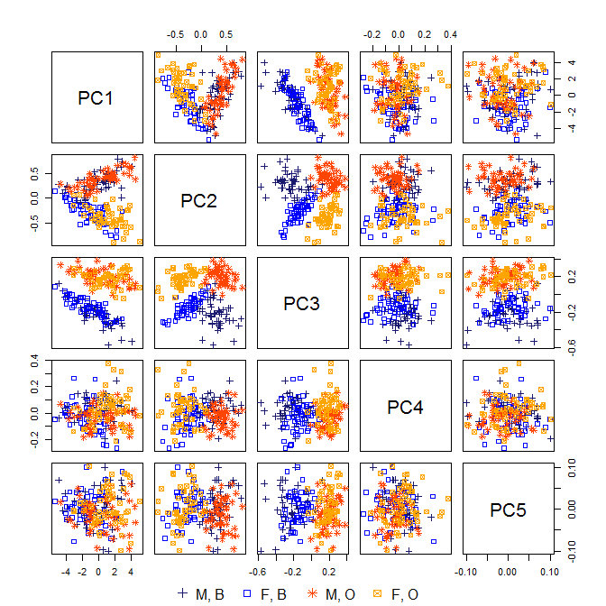
Over 98% of the variance is "explained" by the first two PCs, but in fact if you had actually collected these measurements and were studying them, the third PC is very interesting, because it is closely related to the crab's species. But it is swamped by PC1 (which seems to correspond to the size of the crab) and PC2 (which seems to correspond to the sex of the crab.)

enter image description here

enter image description here

$\endgroup$
3
  • 3
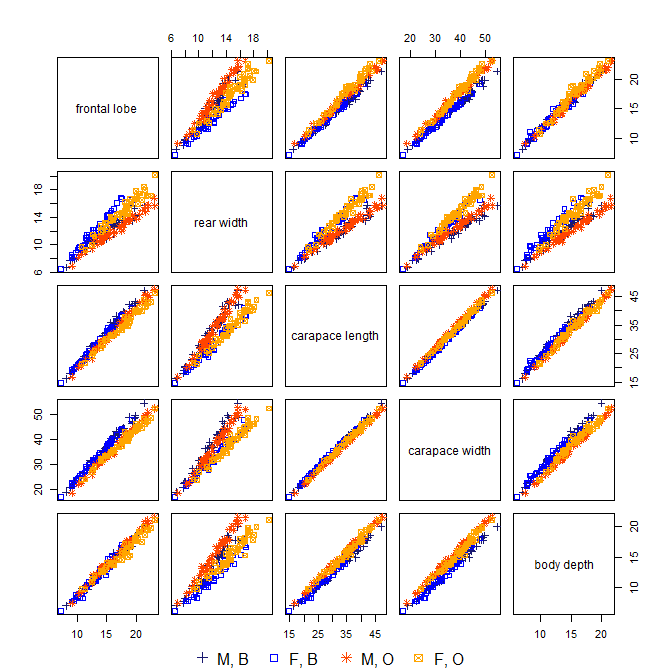
    $\begingroup$ +1, this is a really neat demonstration. I made 2 scatterplot matrices that could be added, if you like. $\endgroup$ Commented Mar 22, 2015 at 1:51
  • 2
    $\begingroup$ @gung: Thanks for adding the scatterplots! I upvoted this answer before, but did not fully appreciate it without seeing the plots. Scatterplot PC2 vs PC3 is really nice: separating both genders and species almost perfectly. I like this example also because it illustrates what happens when all variables are strongly positively correlated (i.e. PC1 explains lots of variance and is basically an average). $\endgroup$
    – amoeba
    Commented Mar 22, 2015 at 22:38
  • 1
    $\begingroup$ Thanks, @amoeba. I really like the way they turned out. I spent a lot of time futzing w/ them (colors, pch, lables, legend). I actually think they're kind of pretty now. You make a good point about PC1. We can also see that there is (probably) a constant coefficient of variation & an interaction by sex &/or species in many of the relationships: small (baby?) crabs tend to have the same values irregardless of sex or species, but as they grow (age?) they become more distinct. Etc. There's lots of neat stuff to see--you can just keep looking at them. $\endgroup$ Commented Mar 23, 2015 at 3:05
10
$\begingroup$

Here are two examples from my experience (chemometrics, optical/vibrational/Raman spectroscopy):

  • I recently had optical spectroscopy data, where > 99% of the total variance of the raw data was due to changes in the background light (spotlight more or less intense on the measured point, fluorescent lamps switched on/off, more or less clouds before the sun). After background correction with the optical spectra of known influencing factors (extracted by PCA on the raw data; extra measurements taken in order to cover those variations), the effect we were interested in showed up in PCs 4 and 5.
    PCs 1 and 3 where due to other effects in the measured sample, and PC 2 correlates with the instrument tip heating up during the measurements.

  • In another measurement, a lens without color correction for the measured spectral range was used. The chromatic aberration lead to distortions in the spectra that accounted for ca. 90 % of total variance of the pre-processed data (captured mostly in PC 1).
    For this data it took us quite a while to realize what exactly had happened, but switching to a better objective solved the problem for later experiments.

(I cannot show details as these studies are still unpublished)

$\endgroup$
5
$\begingroup$

In this talk (slides) the presenters discuss their use of PCA to discriminate between high variability and low variability features.

They actually prefer the low variability features for anomaly detection, since a significant shift in a low variability dimension is a strong indicator of anomalous behavior. The motivating example they provide is as follows:

Assume a user always logs in from a Mac. The "operating system" dimension of their activity would be very low variance. But if we saw a login event from that same user where the "operating system" was Windows, that would be very interesting, and something we'd like to catch.

$\endgroup$
4
$\begingroup$

I have noticed that PCs with low variance are most helpful when performing a PCA on a covariance matrix where the underlying data are clustered or grouped in some way. If one of the groups has a substantially lower average variance than the other groups, then the smallest PCs would be dominated by that group. However, you might have some reason to not want to throw away the results from that group.

In finance, stock returns have about 15-25% annual standard deviation. Changes in bond yields are historically much lower standard deviation. If you perform PCA on the covariance matrix of stock returns and changes in bond yields, then the top PCs will all reflect variance of the stocks and the smallest ones will reflect the variances of the bonds. If you throw away the PCs that explain the bonds, then you might be in for some trouble. For instance, the bonds might have very different distributional characteristics than stocks (thinner tails, different time-varying variance properties, different mean reversion, cointegration, etc). These might be very important to model, depending on the circumstances.

If you perform PCA on the correlation matrix, then you might see more of the PCs explaining bonds near the top.

$\endgroup$
2
  • 1
    $\begingroup$ This answer is very hard to understand if one does not know what stocks, bonds, yields, and returns are. I don't, and so I can't see how your first sentence is related to your second one... $\endgroup$
    – amoeba
    Commented Dec 22, 2014 at 0:40
  • 1
    $\begingroup$ I have made some edits. $\endgroup$
    – John
    Commented Dec 22, 2014 at 1:58
1
$\begingroup$

Here is a very basic and easy to understand example.

This data is a cleaned and simplified version of the data from this study

The grip strength of each hand is measured in kilograms.

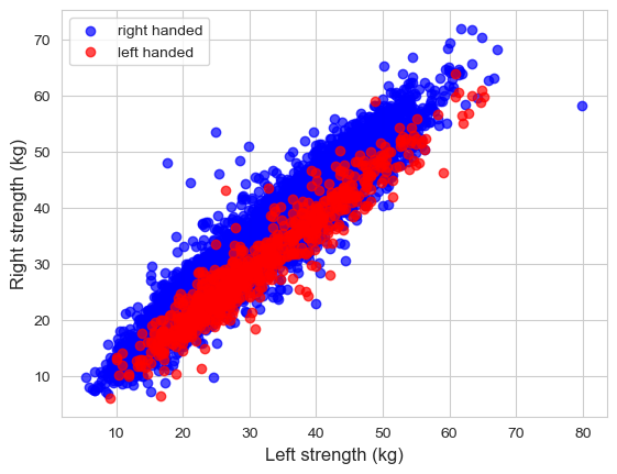
picture of left and right grip strengths, colored by handedness

As is to be expected, the first principle component is very nearly $\begin{bmatrix}1 & 1\end{bmatrix}^\top$ and the second principle component is very nearly $\begin{bmatrix}1 & -1\end{bmatrix}^\top$. However it is the projection onto the second component (i.e. the difference in grip strengths between the left and right hand) which is relevant for discriminating handedness.

$\endgroup$

Your Answer

By clicking “Post Your Answer”, you agree to our terms of service and acknowledge you have read our privacy policy.

Not the answer you're looking for? Browse other questions tagged or ask your own question.