When forcing intercept of 0 in linear regression is acceptable/advisable [duplicate]

Question

I have a regression model to estimate the completion time of a process, based on various factors. I have 200 trials of these processes, where the 9 factors being measured vary widely. When I perform a linear regression of the 9 factors (and all 2 and 3 factor interactions), with no explicit intercept, I get an adjusted R${^2}$ of 0.915, if I force the intercept to 0 I get an adjusted R${^2}$ of 0.953.

My intention of forcing the intercept to 0 was to ensure that trials that completed in very short amounts of time (< 1 second) did not result in predictions of < 0. Setting the intercept to 0 did not help with this.

So my question is threefold. 1) When is it acceptable/advisable to force an intercept? 2) Does the improved R${^2}$ actually mean the model is a better fit (the plot of fitted vs measured did look better)? 3) Is there a way of ensuring the fitted values are all > 0?

Answer 1

It's unusual to not fit an intercept and generally inadvisable - one should only do so if you know it's 0, but I think that (and the fact that you can't compare the $R^2$ for fits with and without intercept) is well and truly covered already (if possibly a little overstated in the case of the 0 intercept); I want to focus on your main issue which is that you need the fitted function to be positive, though I do return to the 0-intercept issue in part of my answer.

The best way to get an always positive fit is to fit something that will always be positive; in part that depends on what functions you need to fit.

If your linear model was largely one of convenience (rather than coming from a known functional relationship that might stem from a physical model, say), then you might instead work with log-time; the fitted model is then guaranteed to be positive in $t$. As an alternative, you might work with speed rather than time - but then with linear fits you may get a problem with small speeds (long times) instead.

If you know your response is linear in the predictors, you can attempt to fit a constrained regression, but with multiple regression the exact form you need will depend on your particular x's (there's no one linear constraint that will work for all $x's$), so it's a bit ad-hoc.

You can also look at GLMs which can be used to fit models which have non-negative fitted values and can (if required) even have $E(Y)=X\beta$.

For example, one can fit a gamma GLM with identity link. You should not end up with a negative fitted value for any of your x's (but you might perhaps have convergence issues in some cases if you force the identity link where it really won't fit).

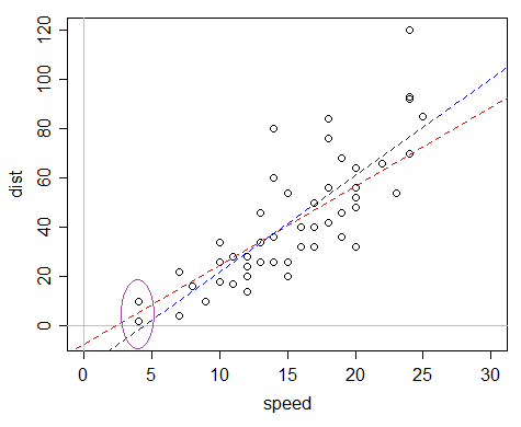
Here's an example: the cars data set in R, which records speed and stopping distances (the response).

One might say "oh, but the distance for speed 0 is guaranteed to be 0, so we should omit the intercept" but the problem with that reasoning is that the model is misspecified in several ways, and that argument only works well enough when the model is not misspecified - a linear model with 0 intercept doesn't fit at all well in this case, while one with an intercept is actually a half-decent approximation even though it's not actually "correct".

The problem is, if you fit an ordinary linear regression, the fitted intercept is quite a way negative, which causes the fitted values to be negative.

The blue line is the OLS fit; the fitted value for the smallest x-values in the data set are negative. The red line is the gamma GLM with identity link -- while having a negative intercept, it only has positive fitted values. This model has variance proportional to mean, so if you find your data are more spread as the expected time grows, it may be especially suitable.

So that's one possible alternative approach that may be worth a try. It's almost as easy as fitting a regression in R.

If you don't need the identity link, you might consider other link functions, like the log-link and the inverse link, which relate to the transformations already discussed, but without the need for actual transformation.

---

Since people usually ask for it, here's the code for my plot:

plot(dist~speed,data=cars,xlim=c(0,30),ylim=c(-5,120))
abline(h=0,v=0,col=8)
abline(glm(dist~speed,data=cars,family=Gamma(link=identity)),col=2,lty=2)
abline(lm(dist~speed,data=cars),col=4,lty=2)

(The ellipse was added by hand afterward, though it's easy enough to do in R as well)

Answer 2

Short answer to question in title: (almost) NEVER. In the linear regression model $$ y = \alpha + \beta x + \epsilon $$, if you set $\alpha=0$, then you say that you KNOW that the expected value of $y$ given $x=0$ is zero. You almost never know that.

$R^2$ becomes higher without intercept, not because the model is better, but because the definition of $R^2$ used is another one! $R^2$ is an expression of a comparison of the estimated model with some standard model, expressed as reduction in sum of squares compared to sum of squares with the standard model. In the model with intercept, the comparison sum of squares is around the mean. Without intercept, it is around zero! The last one is usually much higher, so it easier to get a large reduction in sum of squares.

Conclusion: DO NOT LEAVE THE INTERCEPT OUT OF THE MODEL (unless you really, really know what you are doing).

EDIT (from the comments below): One exception is mentioned elsewhere in the comments (but that is only seemingly an exception, the constant vector 1 is in the column space of the design matrix $X$. Otherwise, such as physical relationships $s=v t$ where there are no constant. But even then, if the model is only approximate (speed is not really constant), it might be better to leave in a constant even if it cannot be interpreted. With non-linear models this becomes more of an issue.

Answer 3

1) It is never acceptable to suppress an intercept except in very rare types of DiD models where the outcome and predictors are actually computed differences between groups (this isn't the case for you).

2). Heck no it doesn't. What it means is that you may have a higher degree of internal validity (e.g. the model fits the data) but probably a low degree of external validity (e.g. the model would be poor in fitting experimental data obtained under similar conditions). This is generally a bad thing.

3) Suppressing the intercept will not necessarily do that, but I assume the predictor was continuous valued. In many situations, process completion times are analyzed using an inverse transform, e.g. $x = 1/t$ where $t$ is the time taken to complete a process. The inverse of the mean of inverse transformed data is called a harmonic mean and represents the average complete time for a task.

$$\mbox{HM} = \frac{1}{\mathbb{E}(x)} = \frac{1}{\mathbb{E}(1/t)} $$

You can also use a parametric exponential or gamma or weibull time-to-event models which are types of models built specifically for predicting completion times. These will give results very similar to the inverse transformed outcomes.

Answer 4

1) Forcing $0$ intercept is advisable if you know for a fact that it is 0. Anything you know a priori, you should use in your model.

One example is the Hubble model for expansion of the Universe (used in Statistical Sleuth):

$$\mbox{Galaxy Speed} = k (\mbox{Distance from Earth}) $$

This model is rather crude, but uses 0 intercept as the consequence of the Big Bang Theory: at time $0$ all the matter is in one place.

On the other hand, the model you're describing will likely need an intercept term.

2) You might or might not get better $R^2_{adj}$, or you may accept null hypothesis for the test for intercept being 0, but both of these are not reasons to remove the intercept term.

3) To ensure positivity of answers, you can sometimes transform the response variable. Log or sqrt might work depending on your data, of course you will need to check the residuals.

Answer 5

It makes sense (actually, is necessary) to leave out the intercept in the second stage of the Engle/Granger cointegration test. The test first estimates a candidate cointegrating relationship via a regression of some dependent variable on a constant (plus sometimes a trend) and the other nonstationary variables.

In the second stage, the residuals of that regression are tested for a unit root to test whether the error actually represents an equilibrium relationship. As the first stage regression contains a constant, the residuals are mean zero by construction. Hence, the second stage unit root test does not need a constant and in fact, the limiting distribution for that unit root test is derived assuming that this constant indeed has not been fitted.

Answer 6

The only way that I know to constrain all fitted values to be greater than zero is to use a linear programming approach and specify that as a constraint.

Answer 7

The actual problem is that a linear regression forcing the intercept=0 is a mathematical inconsistency that should never be done:

It is clear that if y=a+bx, then average(y)=a+average(x), and indeed we can easily realize that when we estimate a and b using linear estimation in Excel, we obtain the above relation

However, if we make arbitrarily a=0, then necessarily b=average(y)/average(x). But this is inconsistent with the minumum squares algorithm. Indeed, you can easily realize that when you estimate b using linear estimation in excel the above relation is not satisfied

Answer 8

It does make pretty much sense in models with categorical covariate. In this case the removal of the intercept results in an equivalent model with just different parametrization:

> data(mtcars)
> mtcars$cyl_factor <- as.factor(mtcars$cyl)
> summary(lm(mpg ~ cyl_factor, data = mtcars))

Call:
lm(formula = mpg ~ cyl_factor, data = mtcars)

Residuals:
    Min      1Q  Median      3Q     Max 
-5.2636 -1.8357  0.0286  1.3893  7.2364 

Coefficients:
            Estimate Std. Error t value Pr(>|t|)    
(Intercept)  26.6636     0.9718  27.437  < 2e-16 ***
cyl_factor6  -6.9208     1.5583  -4.441 0.000119 ***
cyl_factor8 -11.5636     1.2986  -8.905 8.57e-10 ***
---
Signif. codes:  0 ‘***’ 0.001 ‘**’ 0.01 ‘*’ 0.05 ‘.’ 0.1 ‘ ’ 1

Residual standard error: 3.223 on 29 degrees of freedom
Multiple R-squared:  0.7325,    Adjusted R-squared:  0.714 
F-statistic:  39.7 on 2 and 29 DF,  p-value: 4.979e-09

> summary(lm(mpg ~ 0 + cyl_factor, data = mtcars))

Call:
lm(formula = mpg ~ 0 + cyl_factor, data = mtcars)

Residuals:
    Min      1Q  Median      3Q     Max 
-5.2636 -1.8357  0.0286  1.3893  7.2364 

Coefficients:
            Estimate Std. Error t value Pr(>|t|)    
cyl_factor4  26.6636     0.9718   27.44  < 2e-16 ***
cyl_factor6  19.7429     1.2182   16.21 4.49e-16 ***
cyl_factor8  15.1000     0.8614   17.53  < 2e-16 ***
---
Signif. codes:  0 ‘***’ 0.001 ‘**’ 0.01 ‘*’ 0.05 ‘.’ 0.1 ‘ ’ 1

Residual standard error: 3.223 on 29 degrees of freedom
Multiple R-squared:  0.9785,    Adjusted R-squared:  0.9763 
F-statistic: 440.9 on 3 and 29 DF,  p-value: < 2.2e-16

The second example in fact results in the categorical variable being a category-specific intercept, so in reality the intercept isn't actually removed, it just seems so.