How to determine standard errors for treatment and control effects from multiple regression output?

Question

Say I have some data, where a dependent variable, dv, is a function of some independent variable, iv, and a categorical predictor, cat. Here are some example data below generated in R:

set.seed(1) 
a    <- c(1:100)
err  <- rnorm(100, sd=30)
b    <- a + err
c    <- a + err + 20
cat1 <- rep(0,100)
cat2 <- rep(1,100)
iv   <- c(a,a)
dv   <- c(b,c)
cat  <- c(cat1,cat2)
data <- data.frame(dv=dv, iv=iv, cat=cat)

I then model dv as a function of iv and cat with this code:

summary(lm(dv~iv + cat, data=data))

and get the following output

            Estimate Std. Error t value Pr(>|t|)    
(Intercept)  3.94997    4.29669   0.919    0.359    
iv           0.98647    0.06617  14.909  < 2e-16 ***
cat         20.00000    3.81999   5.236  4.2e-07 ***

Now, I want to plot the effect of cat using a standard bar graph- means and errors. So, based on the model, I calculate what the value of dv should be when cat is 0 and when cat is 1, using a common value of iv of 50. For my particular data set, I would get dv values of 53.27339 and 73.27339, for cat levels 0 and 1, respectively.

My question is: Which term from the model should I use for the error bars? Should I just use the standard error estimate of the cat predictor? Or something more complex that integrates the error values of the intercept and iv parameter as well?

Answer 1

Let's start by saving cat as a factor. Then we can play with this a bit to see how it might be done.

cat  <- as.factor(c(cat1,cat2))
data <- data.frame(dv=dv, iv=iv, cat=cat)

By default, R is using reference level coding, which gives you the output you see. An easy way to do this is to center $X$ (iv) on the value you want, so that that becomes the 'intercept', and then fit the model using level means coding (for more information, see my answer to Understanding dummy (manual or automated) variable creation in GLM):

data$iv = data$iv-50
coef(summary(lm(dv~iv + cat+0, data=data)))
# Coefficients:
#      Estimate Std. Error t value Pr(>|t|)    
# iv    0.98647    0.06617   14.91   <2e-16 ***
# cat0 53.27339    2.70134   19.72   <2e-16 ***
# cat1 73.27339    2.70134   27.12   <2e-16 ***

Now the output conveniently gives you exactly what you want. Note that this is the same as what lsmeans (now emmeans) gives you:

library(lsmeans)
lsmeans(m,~iv + cat, at=list(cat=c(0,1), iv=50), data=data )
#  iv cat lsmean  SE  df lower.CL upper.CL
#  50   0   53.3 2.7 197     47.9     58.6
#  50   1   73.3 2.7 197     67.9     78.6
# 
# Confidence level used: 0.95

The question of interest, I suppose, is how this relates to your original output, and why the two standard errors are the same. These values are (slightly) different from SE for the intercept originally. That's because (what was originally) 50 is closer to the mean of iv than the (original) intercept was. What's important to recognize is that the SEs expand as they move away from the mean of $X$ (see my answer to Why does the standard error of the intercept increase the further x¯ is from 0?).

The other thing to understand is that you don't have to somehow integrate the SE for the treatment effect with the baseline SE for the intercept (control arm), because ordinary least squares fits all parameters simultaneously. It doesn't consider the control arm to be ontologically prior and then adjust the estimated treatment away from that. The originally reported SE for the treatment category is the SE for the difference, which is not the same as the SEs for the two constituent arms. (To help clarify these ideas, it may help to read my answer to Is using error bars for means in a within-subjects study wrong?)

---

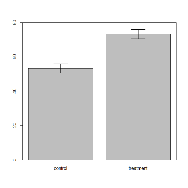
At any rate, it's now easy enough to make a generic bar plot:

windows()
  barplot(c(53.3, 73.3), ylim=c(0,80), names.arg=c("control", "treatment"))
  box()
  arrows(x0=0.7, y0=53.3-2.7, y1=53.3+2.7, code=3, angle=90)
  arrows(x0=1.9, y0=73.3-2.7, y1=73.3+2.7, code=3, angle=90)

Answer 2

Try the lsmeans package from R, which will calculate the expected value and the confidence limits:

lsmeans(mod,~iv + cat, at=list(cat=c(0,1), iv=50), data=data )

 iv cat   lsmean       SE  df lower.CL upper.CL
 50   0 54.09313 3.165838 197 47.84985 60.33642
 50   1 74.09313 3.165838 197 67.84985 80.33642

 Confidence level used: 0.95