Simulating Convergence in Probability to a constant

Question

Asymptotic results cannot be proven by computer simulation, because they are statements involving the concept of infinity. But we should be able to obtain a sense that things do indeed march the way theory tells us.

Consider the theoretical result $$\lim_{n\rightarrow\infty}P(|X_n|>\epsilon) = 0, \qquad \epsilon >0$$

where $X_n$ is a function of $n$ random variables, say identically and independently distributed. This says that $X_n$ converges in probability to zero. The archetypal example here I guess is the case where $X_n$ is the sample mean minus the common expected value of the i.i.d. r.v.'s of the sample,

$$X_n = \frac 1n\sum_{i=1}^nY_i - E[Y_1]$$

QUESTION: How could we convincingly show to somebody that the above relation "materializes in the real world", by using computer simulation results from necessarily finite samples?

Please do note that I specifically chose convergence to a constant.

I provide below my approach as an answer, and I hope for better ones.

UPDATE: Something in the back of my head bothered me -and I found out what. I dug up an older question where a most interesting discussion went on in the comments to one of the answers. In there, @Cardinal provided an example of an estimator that it is consistent but its variance remains non-zero and finite asymptotically. So a tougher variant of my question becomes: how do we show by simulation that a statistic converges in probability to a constant, when this statistic maintains non-zero and finite variance asymptotically?

Answer 1

I think of $P()$ as a distribution function (a complementary one in the specific case). Since I want to use computer simulation to exhibit that things tend the way the theoretical result tells us, I need to construct the empirical distribution function of $|X_n|$, or the empirical relative frequency distribution, and then somehow show that as $n$ increases, the values of $|X_n|$ concentrate "more and more" to zero.

To obtain an empirical relative frequency function, I need (much) more than one sample increasing in size, because as the sample size increases, the distribution of $|X_n|$ changes for each different $n$.

So I need to generate from the distribution of the $Y_i$'s, $m$ samples "in parallel", say $m$ ranging in the thousands, each of some initial size $n$, say $n$ ranging in the tens of thousands. I need then to calculate the value of $|X_n|$ from each sample (and for the same $n$), i.e. obtain the set of values $\{|x_{1n}|, |x_{2n}|,...,|x_{mn}|\}$.

These values can be used to construct an empirical relative frequency distribution. Having faith in the theoretical result, I expect that "a lot" of the values of $|X_n|$ will be "very close" to zero -but of course, not all.

So in order to show that the values of $|X_n|$ do indeed march towards zero in greater and greater numbers, I would have to repeat the process, increasing the sample size to say $2n$, and show that now the concentration to zero "has increased". Obviously to show that it has increased, one should specify an empirical value for $\epsilon$.

Would that be enough? Could we somehow formalize this "increase in concentration"? Could this procedure, if performed in more "sample-size increase" steps, and the one being closer to the other, provide us with some estimate about the actual rate of convergence, i.e. something like "empirical probability mass that moves below the threshold per each $n$-step" of, say, one thousand?

Or, examine the value of the threshold for which, say $90$% of the probability lies below, and see how this value of $\epsilon$ gets reduced in magnitude?

AN EXAMPLE

Consider the $Y_i$'s to be $U(0,1)$ and so

$$|X_n| = \left|\frac 1n\sum_{i=1}^nY_i - \frac 12\right|$$

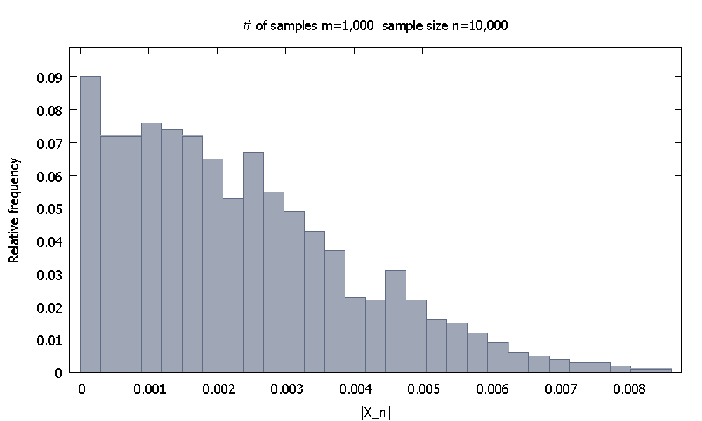
We first generate $m=1,000$ samples of $n=10,000$ size each. The empirical relative frequency distribution of $|X_{10,000}|$ looks like

and we note that $90.10$% of the values of $|X_{10,000}|$ are smaller then $0.0046155$.

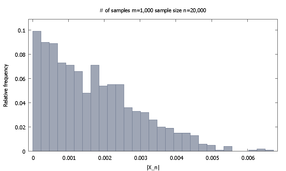
Next I increase the sample size to $n=20,000$. Now the empirical relative frequency distribution of $|X_{20,000}|$ looks like and we note that $91.80$% of the values of $|X_{20,000}|$ are below $0.0037101$. Alternatively, now $98.00$% of values fall below $0.0045217$.

Would you be persuaded by such a demonstration?