9
$\begingroup$

I have a quick question about the central limit theorem. Lets say I measure some value that comes from an arbitrary distribution N times and I repeat this M times. I understand that if I calculcate the mean from the N values I will have a set of M values that follows a normal distribution. But what if I measure the sample standard deviation from N, will my resulting distribution also be normal? Following the derivation of the CLT I do not see this to be the case, but intuitively I think this is true, at least for some distributions. Any light on the issue would be greatly appreciated.

First I will quote the CLT from wiki:

the central limit theorem (CLT) states that, given certain conditions, the arithmetic mean of a sufficiently large number of iterates of independent random variables, each with a well-defined expected value and well-defined variance, be approximately normally distributed.

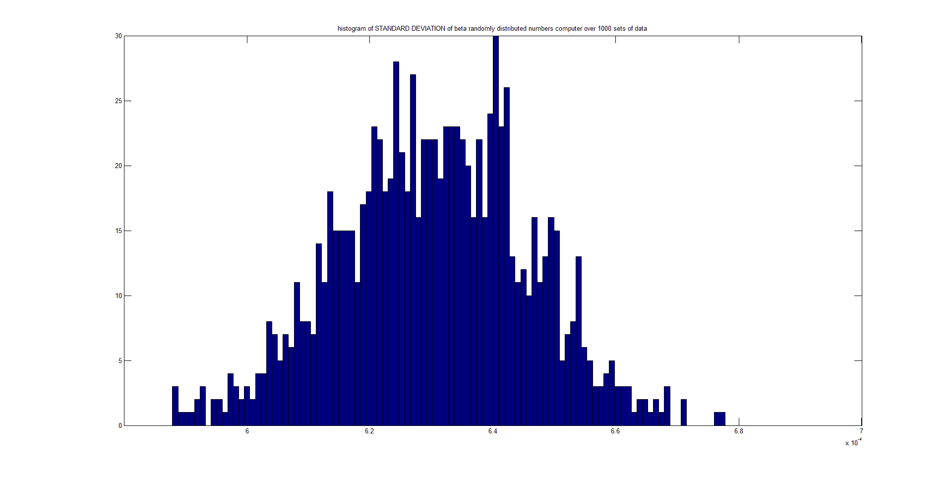
My question then is a variant on the quote from the wiki page: will the the central limit theorem (CLT) state that, given certain conditions, the STANDARD DEVIATION of a sufficiently large number of iterates of independent random variables, each with a well-defined expected value and well-defined variance, be approximately normally distributed? Here is a series of plots I made from random numbers that follow a beta distribution. I have generated 1000 sets of 5000 points each. The first plot is a histogram of the first set. The second is a histogram of the 1000 calculated means, and the 3rd is a histogram of the 1000 calculated std.
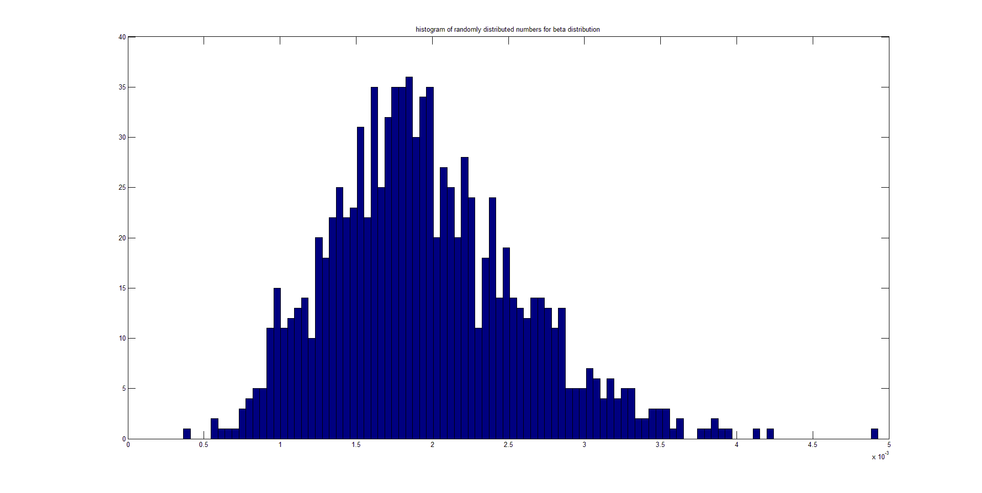
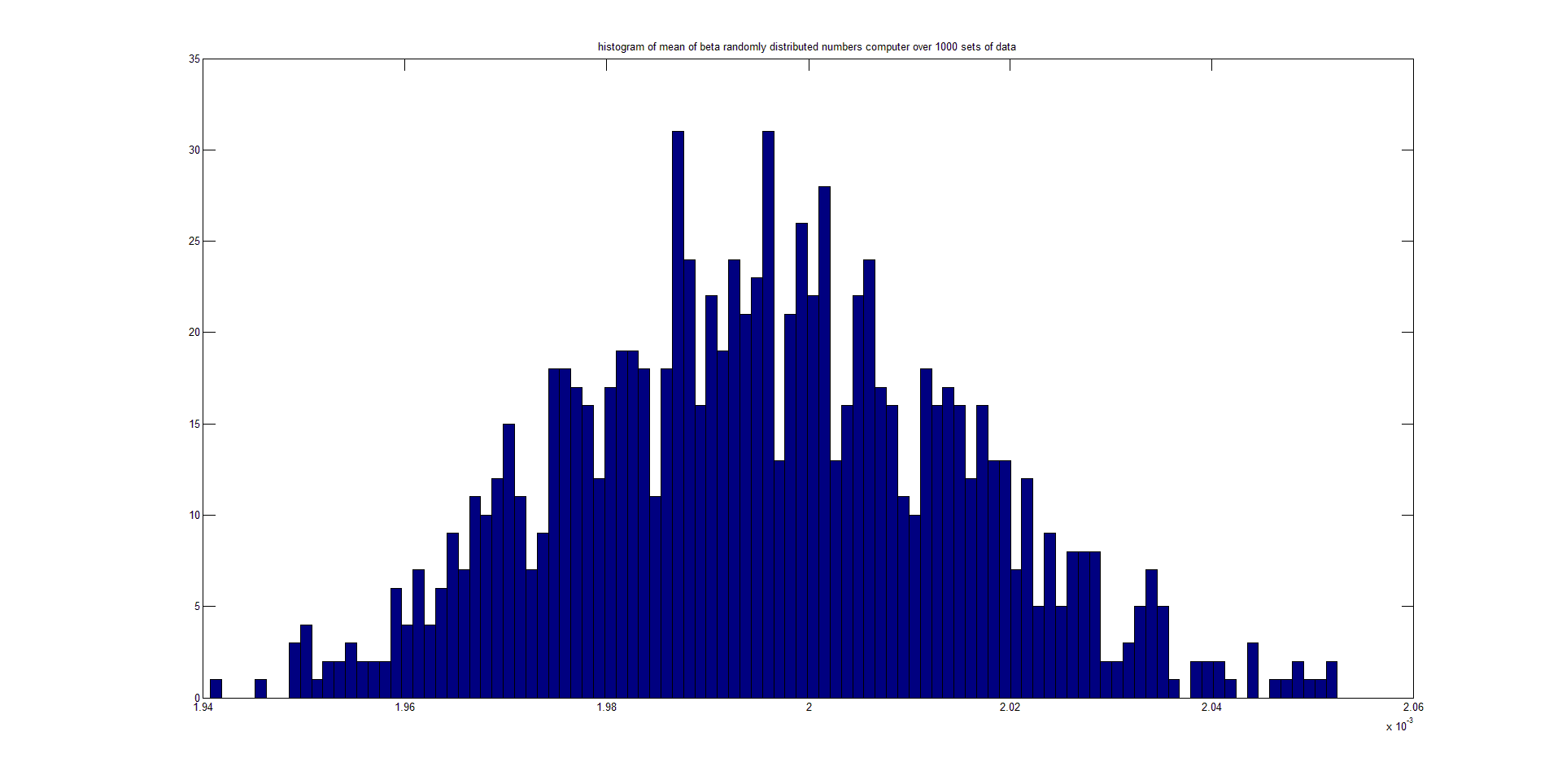
Simulation results

Results 2

Results 3

$\endgroup$
5
  • $\begingroup$ I am sorry, perhaps what I wrote was confusing. The CLT says that if I measure the mean of a set of values a sufficiently large number of times these means will follow a normal distribution. My question is instead if I took the same data set but calculated the sample standard deviation would these values come from a normal distribution? I.e., can the CLT be applied to moments beyond the first moment? Please let me know if this clears up any confusion. Thanks for your help. $\endgroup$
    – user49060
    Commented Jun 26, 2014 at 16:27
  • $\begingroup$ Would mathworld.wolfram.com/StandardDeviationDistribution.html be relevant? $\endgroup$ Commented Jun 26, 2014 at 18:22
  • 4
    $\begingroup$ @Gene That can be used to demonstrate a special case: because the sampling distribution of the SD from a Normal population is $\chi^2$, which asymptotically is Normal, a CLT-like result holds in this case. However, when sampling from a Bernoulli$(1/2)$ variate, the sampling distribution of the SD does not approach normality. $\endgroup$
    – whuber
    Commented Jun 26, 2014 at 18:29
  • 1
    $\begingroup$ "The CLT says that if I measure the mean of a set of values a sufficiently large number of times these means will follow a normal distribution." --- well, actually, that's not quite what any of the versions of the CLT say. The quote from Wikipedia* is closer to accurate (but the claim is strictly speaking false - the CLT doesn't quite say that either). $\quad\quad\quad\quad$ *(not 'wiki' - that's a bit like calling the Library of Congress 'building' when referring to it) $\endgroup$
    – Glen_b
    Commented Jun 27, 2014 at 0:39
  • 1
    $\begingroup$ Under appropriate conditions, you can apply the CLT to the variance (e.g. see p3-4 here). $\endgroup$
    – Glen_b
    Commented Jul 1, 2014 at 1:28

2 Answers 2

11
$\begingroup$

Yes, the sample standard deviation is asymptotically normal. Let the sample standard deviation be $\hat{\sigma} = \sqrt{\frac{1}{n} \sum_{i=1}^n (x_i - \bar{x})^2}$, and let $\sigma$ be the population standard deviation. Let's use the central limit theorem to show that $$ \sqrt{n}(\hat{\sigma} - \sigma) \xrightarrow{d} N(0, V). $$ First write things as $$ \sqrt{n}(\hat{\sigma} - \sigma) = \sqrt{n}\left(\sqrt{ \frac{1}{n} \sum_{i=1}^n (x_i - \bar{x})^2} - \sqrt{\sigma^2} \right)$$ The central limit theorem tells is about how sample moments minus population moments behave. If we didn't have square roots above, we'd just have something like sample moments minus population ones, and we could use the central limit theorem. To get rid of the square roots, let's take a Taylor expansion of the first square root around $\sigma^2$. $$ \sqrt{ \frac{1}{n} \sum_{i=1}^n (x_i - \bar{x})^2} = \sqrt{\sigma^2} + \frac{1}{2\sigma} \left( \frac{1}{n} \sum_{i=1}^n (x_i - \bar{x})^2 - \sigma^2\right) + O\left(\left( \frac{1}{n} \sum_{i=1}^n (x_i - \bar{x})^2 - \sigma^2\right)^2\right) $$ Plugging this into the above, we have $$\sqrt{n}(\hat{\sigma} - \sigma) = \frac{\sqrt{n}}{2 \sigma} \left( \frac{1}{n} \sum_{i=1}^n (x_i - \bar{x})^2 - \sigma^2\right) + O\left(\frac{1}{n^{3/2}} \left(\sum_{i=1}^n (x_i - \bar{x})^2 - \sigma^2\right)^2\right)$$ Rearranging the first term on the right gives $$\frac{\sqrt{n}}{2 \sigma} \left( \frac{1}{n} \sum_{i=1}^n (x_i - \bar{x})^2 - \sigma^2\right) = \frac{1}{2\sigma \sqrt{n}} \sum_{i=1}^n ((x_i - E[X])^2 - \sigma^2) - \frac{\sqrt{n}}{2\sigma}(\bar{x} - E[x])^2 $$ The central limit theorem tells us that under some conditions $\frac{1}{\sqrt{n}} \sum_{i=1}^n (y_i - E[y]) \xrightarrow{d} N(0, \sigma_y^2)$. With $y_i = (x_i - E[x])^2$ and $E[y] = \sigma^2$, then the first term on the right converges in distribution to a normal.

The second term we can write as $\sqrt{n}(\bar{x} - E[x]) (\bar{x} - E[x])$, and since $\sqrt{n}(\bar{x} - E[x]) \xrightarrow{d} N$ and $(\bar{x} - E[x]) \xrightarrow{p} 0$, by Slutsky's lemma, the product converges in probability to 0.

Similarly, we could show that, $\frac{1}{n^{3/2}} \left(\sum_{i=1}^n (x_i - \bar{x})^2 - \sigma^2\right)^2 \xrightarrow{p} 0$, so the remainder from the Taylor expansion vanishes.

This Taylor expansion trick comes up often, so it has a name. It's called the delta method.

$\endgroup$
6
  • 4
    $\begingroup$ I mistrust this argument. I can't put my finger on the error, but I invite you to consider the case where the underlying distribution is Bernoulli$(1/2)$. In this case the sampling distribution of the SD will never be close to Normal: it is always J-shaped and highly negatively skewed. $\endgroup$
    – whuber
    Commented Jun 26, 2014 at 21:06
  • 6
    $\begingroup$ That's a really interesting observation @whuber. The argument breaks down for the Bernoulli(1/2) because then $(x_i - E[x])^2 - \sigma^2= 0$ is constant. Strangely enough, it works for Bernoulli(p) with $p \neq 0.5$. The Bernoulli(1/2) counter-example is a great illustration of why it's important to check those annoying regularity conditions instead of just saying "the central limit theorem tells us that under some conditions ..." like I did. $\endgroup$
    – paul
    Commented Jun 26, 2014 at 23:18
  • 1
    $\begingroup$ I have the suspicion that Slutsky's theorem may not be straightforward to apply when the product of r.v.'s that we consider involves the exact same r.v. Namely, when we have $Y_n$ (converging in probability to zero), and $X_n = \sqrt n Y_n$ (converging in distribution to a random variable), and we consider the product $X_nY_n$. I am looking up various proofs of Slutsky's and I will return. (cc @whuber) $\endgroup$ Commented Jun 27, 2014 at 12:31
  • $\begingroup$ The reason why the Bernoulli(1/2) variable is 'failing' is because it relates to the square of an asymptotic normal distribution with mean 0. The sample variance of the Bernoulli distribution is distributed as $$(X/n)(1-X/n) \quad \text{where } \quad X \sim Binom(n,p)$$ This can also be expressed as $0.25-Y^2$ where $Y = X/n - 0.5$. And this is approximately normal distributed for increasing $n$ and has mean 0 if $p=1/2$. As a result the Taylor expansion needs to use the 2nd order term. A similar situation is in this question about the Delta method stats.stackexchange.com/a/441688 $\endgroup$ Commented Dec 26, 2020 at 18:37
  • $\begingroup$ I think this is misleading. The delta method is applicable in the limit that the function can be approximated by a straight line. So the n will likely need to be significantly larger... In the limit that Gaussian approximates delta function $\endgroup$
    – seanv507
    Commented Dec 28, 2020 at 10:32
1
$\begingroup$

In the comments on Paul's answer Whuber commented that the case of a Bernoulli variable with $p=1/2$ contradicts with his argument. In this question we look further into the Delta method with a graphic. This will provide some intuition and explanation about the (multivariate) Delta method and it explains why the Bernoulli variable is an exception (the only exception along with a degenerate variable).

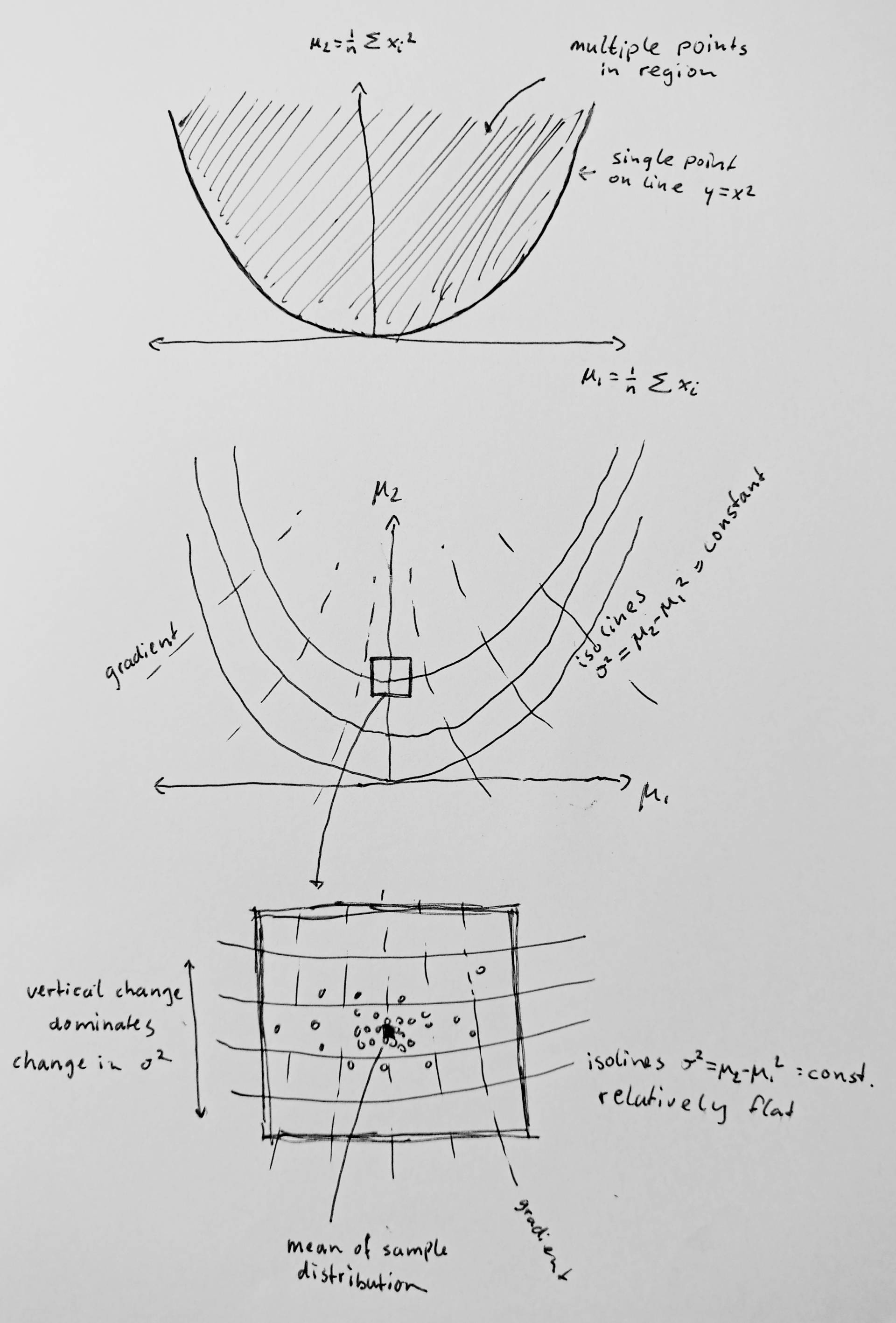
Graphical description and intuition

  1. The standard deviation of a sample equals $\hat\sigma = \sqrt{\hat\mu_2-{\hat\mu_1}^2}$ with $\hat\mu_1 = \frac{1}{n} \sum {x_i}$ and $\hat\mu_2 = \frac{1}{n} \sum {x_i}^2$. We can consider the sample joint distribution of $\mu_1,\mu_2$. The deviation of this sample distribution (scaled by $\sqrt{n}$) should approach a multivariate normal distribution with covariance equal to the covariance of the population distribution of a single point.

  2. On top of the distribution of $\hat\mu_1$ and $\hat\mu_2$ we can consider isolines for $\hat\sigma = \sqrt{\hat\mu_2-{\hat\mu_1}^2} = constant$.

  3. The $\hat\sigma$ is a non-linear function $\hat\mu_1$ and $\hat\mu_2$ but when we consider a small region then the non-linear function can be approximated with a linear function (the delta method does not only require that that a distribution approximates a normal distribution, but also that the variance becomes small).

    If the mean $E(\hat\mu_1) = 0$ (which we can choose without loss of generality by translation of the variable) then $\hat\sigma^2 = \hat\mu_2-{\hat\mu_1}^2$ becomes approximately a normal distributed variable with mean equal to the second moment of the variable and variance equal to the difference of the fourth and second moment $$\sqrt{n}( \hat\sigma^2 - E(\hat\sigma^2)) \xrightarrow[]{P} N(0, E(X^4)-E(X^2)^2)$$

The distribution of $\hat\sigma = \sqrt{\hat\sigma^2}$ can be related to this by the series expansion around $\hat\sigma^2 = E(\hat\sigma^2)$ which is $$\sqrt{\hat\sigma^2} = \sqrt{E(\hat\sigma^2)} + \frac{\hat\sigma^2 - E(\hat\sigma^2)}{2\sqrt{E(\hat\sigma^2)}} + O\left((\hat\sigma^2 - E(\hat\sigma^2))^2\right)$$ and for the limit distribution $$\sqrt{n}( \hat\sigma - \sqrt{E(\hat\sigma^2)}) \xrightarrow[]{P} N\left(0,\frac{ E(X^4)-E(X^2)^2}{4 E(\hat\sigma^2)}\right)$$ This is the limiting distribution. It might not be optimal for approximations of intermediate steps. For instance the mean $\sqrt{E(\hat\sigma^2)}$ is biased and not the same as $E(\hat\sigma)$ (but the bias shrinks to 0 for increasing sample size and that's why it still works as a limit distribution). A similar situation is when you take the logarithm of an approximately normal distributed variable, and you can do better than the Delta method.

enter image description here

The issue with the Bernoulli variable is that the limiting sample distribution of $\hat\mu_1,\hat\mu_2$ is a fully correlated multivariate normal distribution (the population distribution of the $x_i,{x_i}^2$ are just two points and the distribution of the sample mean will be on a straight line between those two points).

In the case of $p=1/2$ (and $x_i = \pm 1$ such that the mean of $x_i$ is zero) the orientation is horizontal; the variance of $\hat\mu_2$ (which is in the vertical direction) is zero, and the first order Delta method does not work (similar question/situation is here). Instead one needs to use the second order Delta method and the distribution becomes related to a chi squared distribution instead of a normal distribution.

$\endgroup$

Your Answer

By clicking “Post Your Answer”, you agree to our terms of service and acknowledge you have read our privacy policy.

Not the answer you're looking for? Browse other questions tagged or ask your own question.