I was using the Linear Discriminant Analysis (LDA) from the scikit-learn machine learning library (Python) for dimensionality reduction and was a little bit curious about the results. I am wondering now what the LDA in scikit-learn is doing so that the results look different from, e.g., a manual approach or an LDA done in R. It would be great if someone could give me some insights here.
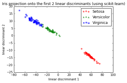
What's basically most concerning is that the scikit-plot shows a correlation between the two variables where there should be a correlation 0.
For a test, I used the Iris dataset and the first 2 linear discriminants looked like this:
IMG-1. LDA via scikit-learn

This is basically consistent with the results I found in the scikit-learn documentation here.
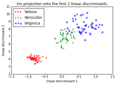
Now, I went through the LDA step by step and got a different projection. I tried different approaches in order to find out what was going on:
IMG-2. LDA on raw data (no centering, no standardization)

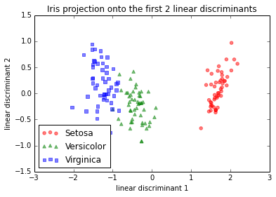
And here would be the step-by-step approach if I standardized (z-score normalization; unit variance) the data first. I did the same thing with mean-centering only, which should lead to the same relative projection image (and which it indeed did).
IMG-3. Step-by-step LDA after mean-centering, or standardization

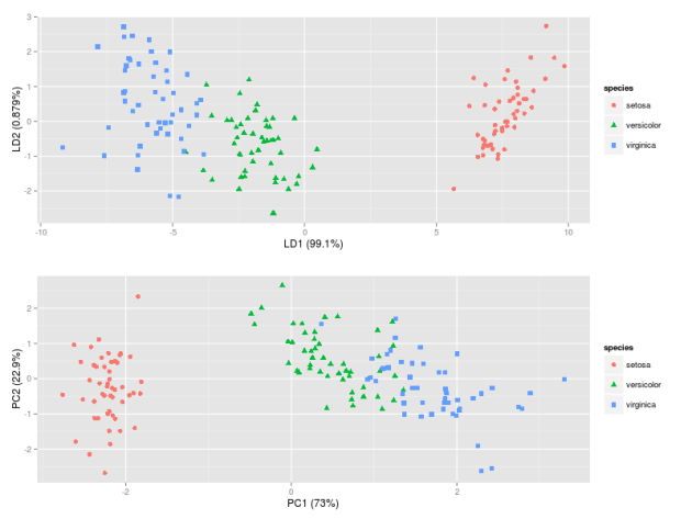
IMG-4. LDA in R (default settings)
LDA in IMG-3 where I centered the data (which would be the preferred approach) looks also exactly the same as the one that I found in a Post by someone who did the LDA in R

Code for reference
I did not want to paste all the code here, but I have uploaded it as an IPython notebook here broken down into the several steps I used (see below) for the LDA projection.
- Step 1: Computing the d-dimensional mean vectors $$\mathbf m_i = \frac{1}{n_i} \sum\limits_{\mathbf x \in D_i}^n \; \mathbf x_k$$
Step 2: Computing the Scatter Matrices
2.1 The within-class scatter matrix $S_W$ is computed by the following equation:
$$S_W = \sum\limits_{i=1}^{c} S_i = \sum\limits_{i=1}^{c} \sum\limits_{\mathbf x \in D_i}^n (\mathbf x - \mathbf m_i)\;(\mathbf x - \mathbf m_i)^T$$2.2 The between-class scatter matrix $S_B$ is computed by the following equation:
$$S_B = \sum\limits_{i=1}^{c} n_i (\mathbf m_i - \mathbf m) (\mathbf m_i - \mathbf m)^T$$ where $\mathbf m$ is the overall mean.Step 3. Solving the generalized eigenvalue problem for the matrix $S_{W}^{-1}S_B$
3.1. Sorting the eigenvectors by decreasing eigenvalues
3.2. Choosing k eigenvectors with the largest eigenvalues. Combining the two eigenvectors with the highest eigenvalues to construct our $d \times k$-dimensional eigenvector matrix $\mathbf W$
Step 5: Transforming the samples onto the new subspace $$\mathbf y = \mathbf W^T \times \mathbf x.$$
