This is one way to go, I will include some numerical calculations using R. Suppose you have a continuous random variable $X$, which is real-valued, and have a density $f(x)$ on the interval $[x_\text{min}, x_\text{max}]$. Then the distribution function $F(x) = \int_{x_\text{min}}^x f(u) \; du $ is continuos and increasing from zero to one on that interval, and the inverse function $Q(p) = F^{-1}(p)$ is also increasing, on the interval $[0, 1]$.
Now use implicit differention on $F(Q(p))=p$ to get $F'(Q(p)) Q'(p)=1$ or
$$
Q'(p) = \frac1{f(x)}.
$$
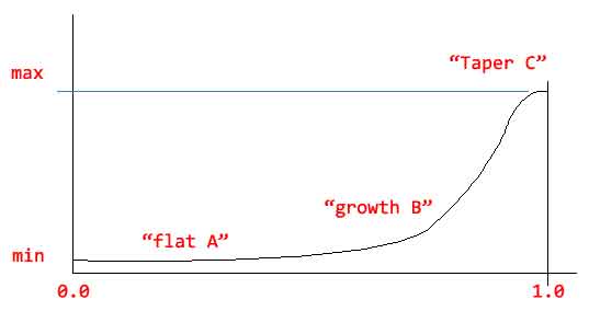
This you can use to read some information from your graph: In the area "flat A" the density is high, "growth B" the density is lower, and "taper C" density increases again. This indicates a bimodal distribution! If you take the interval $x_\text{min}, x_\text{max}$ to be $[0,1]$, you could try to fit some (asymmetric) beta distribution.
To experiment numerically with R, we start to read off some values from your graph. I do this rather haphazardly, you can redo with more precision.
> x
 [1] 0.085 0.090 0.095 0.110 0.150 0.180 0.220 0.250 0.500 0.900 0.980 1.000
> p
 [1] 0.00 0.10 0.20 0.30 0.40 0.50 0.60 0.70 0.80 0.90 0.95 1.00
Fit a monotonic spline:
> Q <- splinefun(p,x,method="monoH.FC")
You can plot these function in R.
Then make a more densely populated table, and use it to plot the inverse function $F(x)$:
> pp  <-  seq(0,1,by=0.01)
> xx <-  Q(pp)
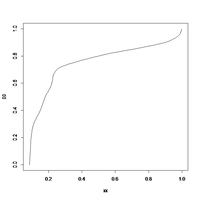
> plot(xx,pp,type="l")
Gives the following plot of the cumulative distribution function:

You could continue, for example using numerical differentiation to find the density, but that I leave for you. From this data we can calculate the expextation of $X$, $\mu=\text{E}(X)$. We use the formula for non-negative random variables
$$
\mu = \int_0^\infty (1-F(t))\; dt
$$
(which in our case reduces to an integral from zero to one because $1-F(t)$ is zero for $t$ larger than one.) In R we can approximate this as
mu <- sum((1-pp))*0.01
mu
1 0.505
When matching to a beta distribution with parameters $a,b$ (refer to wikipedia) we can use then the result that $\mu = \frac{a}{a+b}$, resulting in the choice $a=1.02 b$, or approximately $a=b$. Then you can plot beta distributions for various choices of $a$ ($b$) and see if it matches.


