18
$\begingroup$

I was hoping someone could propose an argument explaining why the random variables $Y_1=X_2-X_1$ and $Y_2=X_1+X_2$, $X_i$ having the standard normal distribution, are statistically independent. The proof for that fact follows easily from the MGF technique, yet I find it extremely counter-intuitive.

I would appreciate therefore the intuition here, if any.

Thank you in advance.

EDIT: The subscripts do not indicate Order Statistics but IID observations from the standard normal distrubution.

$\endgroup$
7
  • $\begingroup$ What is the "MGF technique"? $\endgroup$
    – amoeba
    Commented Aug 20, 2014 at 21:48
  • $\begingroup$ @amoeba It is the use of moment generating functions in order to determine the distribution of a random variable. In my case, I refer to the theorem that $Y_1$ and $Y_2$ are independent if and only if $M(t_1,t_2)=M(t_1,0) \times M(0,t_2) $, $M(t_1,t_2)$ being equal to $E(e^{t_1Y_1+t_2Y_2})$. Choose any other technique and I am confident you will arrive at the same result. $\endgroup$
    – JohnK
    Commented Aug 20, 2014 at 21:54
  • 1
    $\begingroup$ You might find some insight in the closely related thread at stats.stackexchange.com/questions/71260. $\endgroup$
    – whuber
    Commented Aug 20, 2014 at 22:35
  • $\begingroup$ You might get some intuition by considering what happens to each of these if you add some constant, say $\mu$, to each $X$. And what happens if you multiply each $X$ by a constant, say $\sigma$ $\endgroup$
    – Russ Lenth
    Commented Aug 21, 2014 at 0:24
  • 1
    $\begingroup$ Closely related: Reference for the sum and difference of highly correlated variables being almost uncorrelated. $\endgroup$ Commented Aug 21, 2014 at 15:34

4 Answers 4

23
$\begingroup$

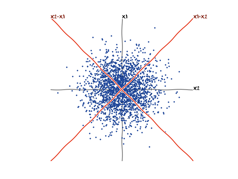
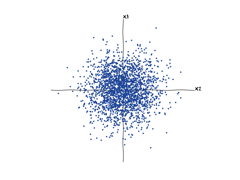
This is standard normal distributed data: scatter plot in first coordinate system Notice that the distribution is circulary symmetric.

When you switch to $Y_1 = X_2 - X_1$ and $Y_2 = X_1 + X_2$, you effectively rotate and scale the axis, like this: scatter plot with rotated coordinate system This new coordinate system has the same origin as the original one, and the axis are orthogonal. Due to the circulary symmetry, the variables are still independent in the new coordinate system.

$\endgroup$
2
  • 4
    $\begingroup$ The result applies even when $X_1$ and $X_2$ are correlated with unit normal margins. So your explanation only covers a subcase of the original result. However, the basic idea here is sound. $\endgroup$
    – Glen_b
    Commented Aug 21, 2014 at 10:25
  • 1
    $\begingroup$ @Glen_b, yes, you're right. I wanted to focus on a simple case, as JohnK already seems to know how to prove the general case, but lacks the intuitive unerstanding. $\endgroup$
    – dobiwan
    Commented Aug 21, 2014 at 11:07
7
$\begingroup$

The result works for $(X_1,X_2)$ jointly normal (i.e. with correlation, $-1<\rho<1$), with common $\sigma$.

If you know a couple of basic results, this is about all you need:

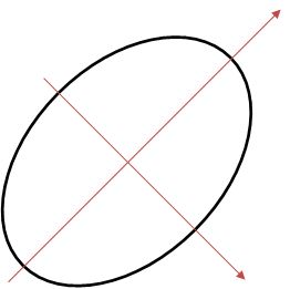
$\quad\quad\quad$ enter image description here

dobiwan's approach is essentially fine - it's just that the result is more general than the case dealt with there.

$\endgroup$
1
  • 3
    $\begingroup$ +1 for stripping down the desired result to the essentials. I will add that for the more general case of joint normality with unequal variances, a rotation of axes by $$\theta = \frac{1}{2}\arctan\left ( \frac{2\rho\cdot\sigma_1\sigma_2}{\sigma_1^2 - \sigma_2^2}\right )$$ instead of the $\pm \frac{\pi}{4}$ implicit in $(X_1,X_2) \to (X_1+X_2. X_1-X_2)$ produces independent normal random variables. $\endgroup$ Commented Aug 21, 2014 at 12:08
6
$\begingroup$

The result you claim to be true is not true in general, not even for the case when all that is known is that $X_1$ and $X_2$ are normal random variables with identical variance, but the result does hold for the usual interpretation of the condition you stated later:

The subscripts do not indicate Order Statistics but observations from the standard normal distrubution.

The usual interpretation of the last few words in this statement is, of course, that $X_1$ and $X_2$ are independent (normal) random variables, and hence jointly normal random variables.

For jointly normal random variables with identical variance, it is true that $X_1+X_2$ and $X_1-X_2$ are independent (normal) random variables (with, in general, unequal variances), and the intuitive explanation for this is best given in Glen_b's answer. For your special case of $X_1$ and $X_2$ being independent as well, dobiwan's answer, which you have accepted, is simplest, and indeed reveals that any rotation of the axes, not just by the $\pm \frac{\pi}{4}$ implicit in the transformation $(X_1,X_2)\to (X_1+X_2, X_1-X_2)$, will yield independent random variables.


What can be said in general? In everything I say below, please bear in mind that $X$ and $Y$ have the same variance, no matter what other properties might be attributed to them.

If $X$ and $Y$ are any random variables (note: not necessarily normal) with identical variance, then $X+Y$ and $X-Y$ are uncorrelated random variables (that is, they have zero covariance). This is because the covariance function is bilinear: $$\begin{align} \operatorname{cov}(X+Y, X-Y) &= \operatorname{cov}(X,X) - \operatorname{cov}(X,Y) + \operatorname{cov}(Y,X) - \operatorname{cov}(Y,Y)\\ &= \operatorname{var}(X) - \operatorname{cov}(X,Y) + \operatorname{cov}(X,Y) - \operatorname{var}(Y)\\ &= 0. \end{align}$$ Here we have used the fact that $\operatorname{cov}(X,X)$ is just the variance $\operatorname{var}(X)$ of $X$ (and similarly for $Y$) and, of course, $\operatorname{cov}(Y,X) = \operatorname{cov}(X,Y)$. Note that this result holds when $X$ and $Y$ are (marginally) normal random variables but not necessarily jointly normal random variables. (If you are not familiar with this notion of marginal normality not being the same as joint normality, see this great answer by cardinal). In the special case when $X$ and $Y$ are jointly normal (but not necessarily independent) normal random variables, so are $X+Y$ and $X-Y$ jointly normal, and since their covariance is $0$, $X+Y$ and $X-Y$ are independent random variables.

$\endgroup$
0
2
$\begingroup$

I first argue for general identically distributed $X_1,X_2$ that the conditional mean of $Y_1$ conditional on $Y_2$ is constant $0$. Based on this, I argue that the covariance of  $Y_1,Y_2$ is 0. Then, under normality, zero covariance implies independence.

The conditional mean

Intuition: $X_1+X_2=y$ does not imply anything about which component contributed more to the sum (e.g., $X_1=x, X_2 = y-x$ is as likely as $X_1 = y-x, X_2=x$). Thus, the expected difference must be 0.

Proof: $X_1$ and $X_2$ have identical distribution and $X_1+X_2$ is symmetric with respect to the indexing. Thus, for symmetry reasons, the conditional distribution $X_1 \mid Y_2 = y$ must be equal to the conditional distribution $X_2 \mid Y_2 = y$. Hence, the conditional distributions also have the same mean, and \begin{equation} \mathbb{E}(Y_1 \mid Y_2 = y) = \mathbb{E}(X_1 - X_2 \mid X_1+X_2 = y) \\ = \mathbb{E}(X_1 \mid X_1+X_2 = y) - \mathbb{E}(X_2 \mid X_1+X_2 = y)= 0. \end{equation}

(Caveat: I did not consider the possibility that the conditional mean might not exist.)

Constant conditional mean implies zero correlation/covariance

Intuition: correlation measures how much $Y_1$ tends to increase when $Y_2$ increases. If observing $Y_2$ never changes our mean of $Y_1$, $Y_1$ and $Y_2$ are uncorrelated.

Proof: By definition, covariance is \begin{equation} Cov(Y_1,Y_2) = \mathbb{E}\left[\left(Y_1 - \mathbb{E}(Y_1)\right)\left(Y_2 -\mathbb{E}(Y_2) \right)\right] \end{equation} to this expectation, we apply the law of iterated expectations: take the expectation of the conditional expectation conditional on $Y_2$: \begin{equation} = \mathbb{E}\left[\mathbb{E}\left[\left(Y_1 - \mathbb{E}(Y_1)\right)\left(Y_2 -\mathbb{E}(Y_2) \right) \mid Y_2\right]\right] = \mathbb{E}\left[(Y_2 - \mathbb{E}(Y_2))\mathbb{E}\left[Y_1 - \mathbb{E}(Y_1) \mid Y_2\right] \right]. \end{equation} Recall that the conditional mean was shown to be independent of $Y_2$ and thus the expression simplifies as \begin{equation} = \mathbb{E}\left[(Y_2 - \mathbb{E}(Y_2))\mathbb{E}\left[Y_1-\mathbb{E}(Y_1)\right]\right] \end{equation} but the inner expectation is $0$ and we get \begin{equation} = \mathbb{E}\left[(Y_2 - \mathbb{E}(Y_2))\times0\right] = 0. \end{equation}

Independence

Just by assuming identical distributions for $X_1,X_2$, it was shown that $Y_1$ and $Y_2$ are uncorrelated. When $X_1,X_2$ are jointly normal (for example, iid. normal as in the question), their linear combinations $Y_1,Y_2$ are also jointly normal and thus uncorrelatedness implies independence.

$\endgroup$

Your Answer

By clicking “Post Your Answer”, you agree to our terms of service and acknowledge you have read our privacy policy.

Not the answer you're looking for? Browse other questions tagged or ask your own question.