R and JMP produce different regression results due to sum of squares calculation and other factors

Question

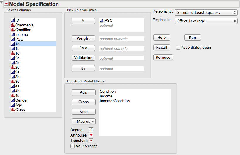
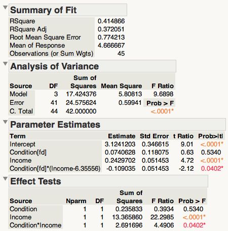
I recently started transitioning from JMP to R and to get started, I've been trying to reproduce some of my old JMP results in R. However, when I run a multiple regression with one continuous variable (income) and one categorical variable (condition) predicting a continuous variable (psc), the results from the 2 programs differ.

Here's my JMP model and results:

And here's my R code and results:

> library(plyr)

> # load data files
> online <- read.csv('r_online.csv')
> paper <- read.csv('r_paper.csv')

> # define conditions for online data
> online$condition <- NA
> levels(online$condition) <- c('wc','fd')

> online[!is.na(online$Ntrl1), 'condition'] <- 'wc'
> online[!is.na(online$Ntrl3), 'condition'] <- 'fd'

> online$condition <- factor(online$condition)

> # merge online and paper data
> mydata <- rbind.fill(online, paper)

> # exclude dropped data
> mydata <- subset(mydata, Class < 5)

> # calcualte psc
> psc <- ((8-mydata$PSF1r)+(8-mydata$PSF2r)+mydata$PSF3+(8-mydata$PSF4r)+(8-mydata$PSF5r)+mydata$PSF6)/6
> mydata$psc <- psc

> # save income and condition as values
> income <- mydata$Income
> condition <-mydata$condition

> # psc by income and condition
> psc.income.regress <- lm(psc ~ income * condition)
> summary(psc.income.regress)

Call:
lm(formula = psc ~ income * condition)

Residuals:
    Min      1Q  Median      3Q     Max 
-1.7275 -0.3585  0.0731  0.5122  1.1602 

Coefficients:
                   Estimate Std. Error t value Pr(>|t|)    
(Intercept)         3.89116    0.50804   7.659 1.96e-09 ***
income              0.13393    0.07494   1.787   0.0813 .  
conditionwc        -1.53409    0.69323  -2.213   0.0325 *  
income:conditionwc  0.21807    0.10291   2.119   0.0402 *  
---
Signif. codes:  0 ‘***’ 0.001 ‘**’ 0.01 ‘*’ 0.05 ‘.’ 0.1 ‘ ’ 1

Residual standard error: 0.7742 on 41 degrees of freedom
  (4 observations deleted due to missingness)
Multiple R-squared:  0.4149,    Adjusted R-squared:  0.3721 
F-statistic:  9.69 on 3 and 41 DF,  p-value: 5.854e-05

So, R-squared, R-squared Adjusted, Overall F, Overall p, and p and t for the interaction are the same in both R and JMP, but p and t for the main effects and all of the Estimates are different.

I did some reading and found that this occurs because JMP calculates Type-III sums of squares, while R calculates Type-I SS. So far, though, I haven't been able to figure out how to get R to calculate Type-III SS in the same way as JMP.

One site said that I could get Type-III SS by changing the last part of my R code to this:

> ### alternative method suggested for getting type-III SS ###
> options(contrasts=c("contr.sum","contr.poly"))
> psc.income.regress <- lm(psc ~ income * condition)
> drop1(psc.income.regress,~.,test="F")

Single term deletions

Model:
psc ~ income * condition
                 Df Sum of Sq    RSS      AIC F value    Pr(>F)    
<none>                        24.576 -19.2208                      
income            1   13.3659 37.941  -1.6778 22.2985 2.729e-05 ***
condition         1    2.9354 27.511 -16.1434  4.8972   0.03253 *  
income:condition  1    2.6917 27.267 -16.5438  4.4906   0.04018 *  
---
Signif. codes:  0 ‘***’ 0.001 ‘**’ 0.01 ‘*’ 0.05 ‘.’ 0.1 ‘ ’ 1


> summary(psc.income.regress)

Call:
lm(formula = psc ~ income * condition)

Residuals:
    Min      1Q  Median      3Q     Max 
-1.7275 -0.3585  0.0731  0.5122  1.1602 

Coefficients:
                  Estimate Std. Error t value Pr(>|t|)    
(Intercept)        3.12412    0.34662   9.013 2.82e-11 ***
income             0.24297    0.05145   4.722 2.73e-05 ***
condition1         0.76704    0.34662   2.213   0.0325 *  
income:condition1 -0.10904    0.05145  -2.119   0.0402 *  
---
Signif. codes:  0 ‘***’ 0.001 ‘**’ 0.01 ‘*’ 0.05 ‘.’ 0.1 ‘ ’ 1

Residual standard error: 0.7742 on 41 degrees of freedom
  (4 observations deleted due to missingness)
Multiple R-squared:  0.4149,    Adjusted R-squared:  0.3721 
F-statistic:  9.69 on 3 and 41 DF,  p-value: 5.854e-05

Now all the estimates for income, interaction, and the intercept are the same in R as in JMP, but condition is still different.

Another person suggested that I recode my conditions as numeric contrasts (instead of having them as factors) and center everything, so I changed the end of my code to this:

> ### 2nd alternative method: change condition to numeric contrast and center variables ###
> condition_c <- ifelse(condition == 'fd', +.5, -.5)
> condition_c <- scale(condition_c, scale=F,center=T)
> income_c <- scale(income,scale=F,center=T)
> psc.income.regress <- lm(psc ~ income_c * condition_c)
> summary(psc.income.regress)

Call:
lm(formula = psc ~ income_c * condition_c)

Residuals:
    Min      1Q  Median      3Q     Max 
-1.7275 -0.3585  0.0731  0.5122  1.1602 

Coefficients:
                     Estimate Std. Error t value Pr(>|t|)    
(Intercept)           4.67891    0.11588  40.379  < 2e-16 ***
income_c              0.22739    0.05241   4.338 9.13e-05 ***
condition_c           0.14813    0.23615   0.627   0.5340    
income_c:condition_c -0.21807    0.10291  -2.119   0.0402 *  
---
Signif. codes:  0 ‘***’ 0.001 ‘**’ 0.01 ‘*’ 0.05 ‘.’ 0.1 ‘ ’ 1

Residual standard error: 0.7742 on 41 degrees of freedom
  (4 observations deleted due to missingness)
Multiple R-squared:  0.4149,    Adjusted R-squared:  0.3721 
F-statistic:  9.69 on 3 and 41 DF,  p-value: 5.854e-05

Doing this, the p and t values for the interaction and condition become the same as in JMP, but now income and all the estimates are different.

I've tried to be as thorough as I can in trying finding an answer on my own, but I've run out of ideas so any help would be immensely appreciated. All relevant R files can be found here: https://www.dropbox.com/s/eoup5im2iko1ro6/R.zip?dl=0

Answer 1

Figured it out. After condition <- mydata$condition in my original R code, adding these lines (instead of what I had there originally) makes the R results identical to the JMP results:

  # change contrasts from the R defaults:
options(contrasts=c("contr.sum", "contr.poly")) 
  # center income:
income_c <- scale(income, scale=F, center=T) 
  # use centered income instead of uncentered income, which I was using before:
psc.income.regress <- lm(psc ~ income_c * condition) 
  # gives the coefficients, t, and p seen in JMP output:
summary(psc.income.regress) 
  # gives the SS and F seen in JMP output:
drop1(psc.income.regress, ~., test="F") 

Answer 2

JMP centers polynomials by default. You can override that default by unclicking that option under the red triangle by "Model Specification" in the "Fit Model" dialog box. Doing so will produce the same results for the Type III sums-of-squares as R, when you use the car package and appropriate contrasts. In other words, if you wish to reproduce JMP's default results in R, you must center your numerical predictor in R first. If you wish to reproduce R's default in JMP, you must unselect the "Center Polynomials" option in JMP first.