30
$\begingroup$

I was attempting to simulate injection of random points within a circle, such that any part of the circle has the same probability of having a defect. I expected the count per area of the resulting distribution to follow a Poisson distribution if I break up the circle into equal area rectangles.

Since it requires only placing points within a circular area, I injected two uniform random distributions in polar coordinates: $R$ (radius) and $\theta$ (polar angle).

But after doing this injection, I clearly get more points in the center of the circle compared to the edge.

enter image description here

What would be the correct way to perform this injection across the circle such that the points are randomly distributed across the cirlce?

$\endgroup$
1

4 Answers 4

43
$\begingroup$

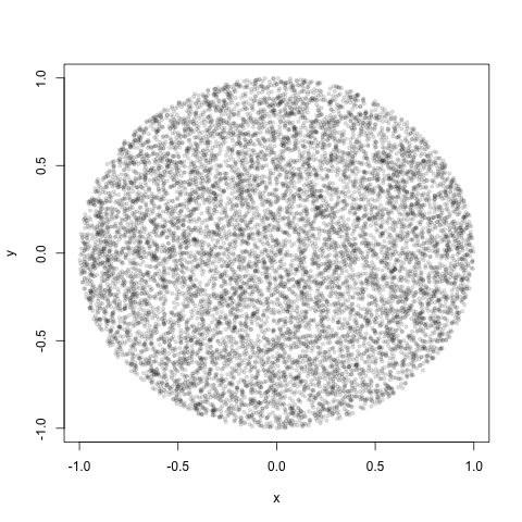
You want the proportion of points to be uniformly proportional to area rather than distance to the origin. Since area is proportional to the squared distance, generate uniform random areas and take their square roots; scale the results as desired. Combine that with a uniform polar angle.

This is quick and simple to code, efficient in execution (especially on a parallel platform), and generates exactly the prescribed number of points.

Example

This is working R code to illustrate the algorithm.

n <- 1e4
rho <- sqrt(runif(n))
theta <- runif(n, 0, 2*pi)
x <- rho * cos(theta)
y <- rho * sin(theta)
plot(x, y, pch=19, cex=0.6, col="#00000020")

enter image description here

$\endgroup$
1
  • $\begingroup$ A less efficient but more amusing answer appears (implicitly) at stats.stackexchange.com/a/520811/919: generate uniformly distributed points on the surface of a three-sphere in $\mathbb{R}^4$ (by scaling a four-dimensional standard Normal variable) and simply retain their first two components! $\endgroup$
    – whuber
    Commented Apr 22, 2021 at 19:01
7
$\begingroup$

Rejection Sampling can be used. This means we can sample from 2D uniform distribution, and select samples that satisfy the disc condition.

Here is an example.

x=runif(1e4,-1,1)
y=runif(1e4,-1,1)

d=data.frame(x=x,y=y)
disc_sample=d[d$x^2+d$y^2<1,]
plot(disc_sample)

enter image description here

$\endgroup$
3
  • 4
    $\begingroup$ This is a good alternative to the approach taken by the OP. Simple and efficient. It doesn't really address the question, though, which concerns how to modify the polar coordinate method to produce uniformly distributed variates. Why might we care? Because of the implications: once you know how to generate uniformly distributed points in polar coordinates, you can use rejection sampling (and other familiar methods) in polar coordinates to sample from regions that might be prohibitively complicated to sample in Cartesian coordinates (think of hypocycloids, for instance). $\endgroup$
    – whuber
    Commented Sep 21, 2017 at 18:13
  • 1
    $\begingroup$ Note, too, that you haven't generated 10,000 points in the disk: the number of points is a random value near $\pi/4$ times 10,000. There are efficient ways around this, but implementing them complicates the algorithm. $\endgroup$
    – whuber
    Commented Sep 21, 2017 at 18:15
  • 1
    $\begingroup$ @whuber thanks for educating me by commenting my answer! $\endgroup$
    – Haitao Du
    Commented Sep 21, 2017 at 18:18
7
$\begingroup$

I'll give you a general n-dimensional answer that works for two-dimensional case too, of course. In three dimensions an analog of a disk is a volume of a solid ball (sphere).

There are two approaches I'm going to discuss. One of them I would call "precise", and you'll get a complete solution with it in R. The second one I call heuristic, and it's only the idea, no complete solution is provided.

"Precise" solution

My solution is based on Marsaglia and Muller's works. Basically, it happens so that the Gaussian vector normalized to its norm would give you the uniformly distributed points on a d-dimensional hypersphere:

enter image description here

It's the same as uniformely distributed points on a circle in two dimensions. To extend this to the entire surface of a disk, you need to further scale them by radius. The square of a radius is from uniform distribution in two dimensions, or raised to power $d$ in d-dimensions. So, you raise to power $1/d$ a uniform random number to get the properly distributed radius. Here's a complete code in R for two dimensions, which you can easily extend to any number of dimensions:

n <- 1e4
rho <- sqrt(runif(n))
# d - # of dimensions of hyperdisk
d = 2
r = matrix(rnorm(n*d),nrow=n,ncol=d)
x = r/rep(sqrt(rowSums(r^2))/rho,1)
plot(x[,1], x[,2], pch=19, cex=0.6, col="#00000020")
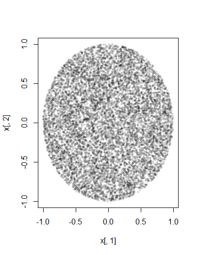
enter image description here

Here's a code snippet for 3d case, i.e. a solid ball:

library(scatterplot3d)
n <- 1e3
# d - # of dimensions of hyperdisk

d=3
rho <- (runif(n))^(1/d)
r = matrix(rnorm(n*d),nrow=n,ncol=d)
x = r/rep(sqrt(rowSums(r^2))/rho,1)

scatterplot3d(x[,1], x[,2], x[,3])
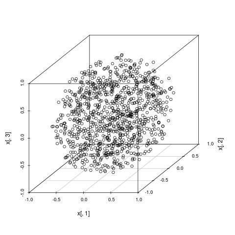
enter image description here

Heuristic approach

This approach is based on a not so obvious fact that the ration of the volume of the unit hypersphere over the volume of a unit hypercube that encloses it shrinks to zero when the number of dimensions increases to infinity. This can easily be seen from the expression for a volume of a hypersphere: $$V_n(R) = \frac{\pi^\frac{n}{2}}{\Gamma\left(\frac{n}{2} + 1\right)}R^n$$ Here, you can see how the coefficient in front of $R^n$ quickly decreases to zero. This is another manifestation of the phenomenon that is linked to what's known as a dimensionality curse in machine learning.

Why is this relevant to our problem at hand? Suppose, you want to generate d random uniform numbers, these would the random points inside d-dimensional hypercube. Next, you apply rejection sampling to pick the points inside the hypersphere (aka n-ball): $\sum_{i=1}^d x_i^2<R^2$. The problem is that for high number of dimensions d, almost all points will be outside the sphere! You'll end up throwing out vast majority of your samples.

The solution I propose is to use the rejection sampling with oversampling the points near the center. It turns out that if you were watching one of the cartesian coordinates of the random uniform sample from inside the ball, its distribution would be converging to a Gaussian with variance $\frac 1 {\sqrt{d+2}}$. So, instead of picking points uniformly from the cube, we be sampling the cartesian coordinate using the Gaussian, then apply rejection sampling on them. This way we would not be wasting as many generated random variates. This would be a form of importance sampling technique.
$\endgroup$
4
  • $\begingroup$ @Silverfish, you're right, I fixed the language $\endgroup$
    – Aksakal
    Commented May 6, 2019 at 20:32
  • 1
    $\begingroup$ @Silverfish, it's slow due to use of Gaussian variates, but could be faster than simple rejection sampling in high dimensional case, which is not obvious to many, though it's a different subject $\endgroup$
    – Aksakal
    Commented May 6, 2019 at 20:52
  • $\begingroup$ (1) In the 3D example why are you taking the square root of a uniform variate for the radius and not the cube root? (2) You seem to be claiming one should raise the square of the radius to $1/d,$ but don't you mean the radius itself, unsquared? (3) In what way is the rejection sampling approach any better than the previous approach, which needs only $d$ iid Gaussian variates (with no rejection)? $\endgroup$
    – whuber
    Commented May 6, 2019 at 21:28
  • $\begingroup$ @whuber, I was copy pasting, corrected a typo on cube power. If we use Gaussian then rejection sampling is not better, so we'd have to use something bell shaped that is faster than Gaussian, you're right $\endgroup$
    – Aksakal
    Commented May 6, 2019 at 21:43
2
$\begingroup$

Here is an alternative solution in R:

n <- 1e4
## r <- seq(0, 1, by=1/1000)
r <- runif(n)
rho <- sample(r, size=n, replace=T, prob=r)
theta <- runif(n, 0, 2*pi)
x <- rho * cos(theta)
y <- rho * sin(theta)
plot(x, y, pch=19, cex=0.6, col="#00000020")

enter image description here

$\endgroup$
4
  • 5
    $\begingroup$ Can you explain this answer in plain English? We aren't really a code help site, & code-only answers should be discouraged. $\endgroup$ Commented Sep 21, 2017 at 17:54
  • 6
    $\begingroup$ This solution is intriguing. Unfortunately it is not quite correct, although the plot looks fine. The reason is that it limits the radii in the sample to a discrete set of values equally spaced between $0$ and $1$. This is not the same as the intended distribution. In particular, it is singular: it doesn't even have a PDF! If you're not convinced, rerun it with r <- seq(0, 1, by=1/10) instead to see its discrete nature more clearly. $\endgroup$
    – whuber
    Commented Sep 21, 2017 at 18:01
  • 1
    $\begingroup$ @whuber Thanks for pointing that out. It is actually my main idea of the solution. My approach was to generate many uniform circles with varying radii, and, for each circle, the number of points is proportional to the length of its radius. Therefore, on a unit length of circles with different radii, the number of points is the same. To avoid the discrete nature, we could sample r from Uniform(0,1). $\endgroup$
    – Q_Li
    Commented Oct 9, 2017 at 19:58
  • 1
    $\begingroup$ (+1) With your edit, the method becomes clearer. It's quite clever: by sampling $r$ and then sampling $\rho$ uniformly in $[0,r],$ you effectively are sampling $\rho^2$ from a uniform $[0,1]$ distribution. Although that's not the most efficient solution in the present case, it illustrates an interesting technique the potentially, in some other circumstance, could be effective and illuminating. $\endgroup$
    – whuber
    Commented Sep 29, 2020 at 20:48

Your Answer

By clicking “Post Your Answer”, you agree to our terms of service and acknowledge you have read our privacy policy.

Not the answer you're looking for? Browse other questions tagged or ask your own question.