I am working on a dataset with a continuous response (which could be dichotomized), one continuous covariate, and multiple categorical variables. The continuous covariate (weight) is directly correlated to the response, and must be accounted for so that we can determine which of the categorical variables are most influential to the response. Here is example data.
Each row is an individual subject, with the continuous response, the covariate of underlying primary importance (weight), then 10 categorical variables that are to be tested (individuals can score yes = 1 to multiple categories).
My first thought in working with this data was a linear model, with stepwise elimination of categorical variables.
lm(Response~Weight+var1+var2...+var11)
However, I believe there is extensive collinearity, since some variables may be eliminated early, but then are significant if you add them back into the model at the end. I'm curious if there is a better way to approach this data in R, that may help sort through which of the variables are of most importance to influencing the response. My two thoughts are
1) Building a single model with the continuous covariate and 5 categorical variables that were selected to be of most interest before the study, and refrain from any stepwise reduction of this model
2) Some sort of princicpal component regression, which I know little about at this point and thus wanted to ask advice before proceeding down that path
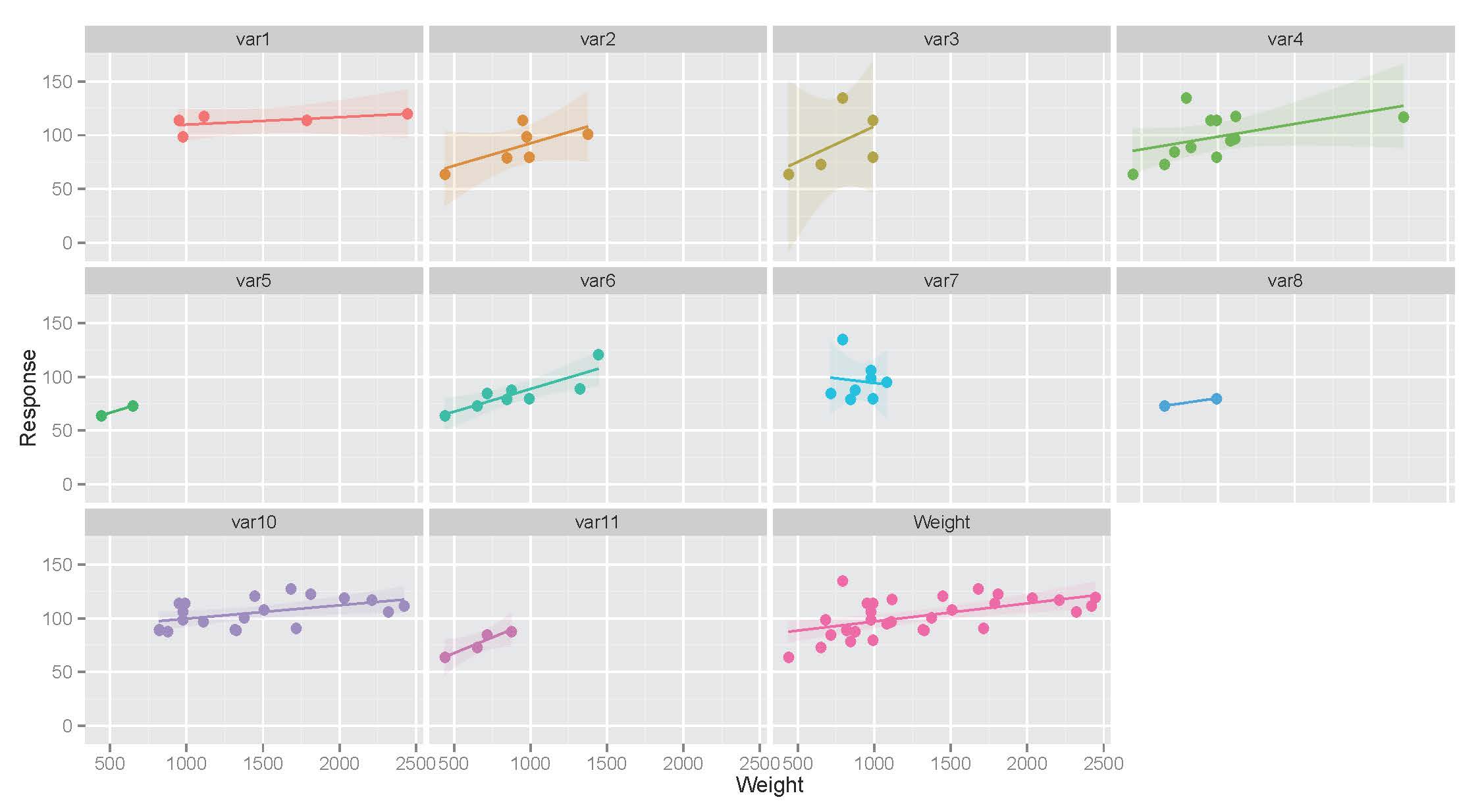
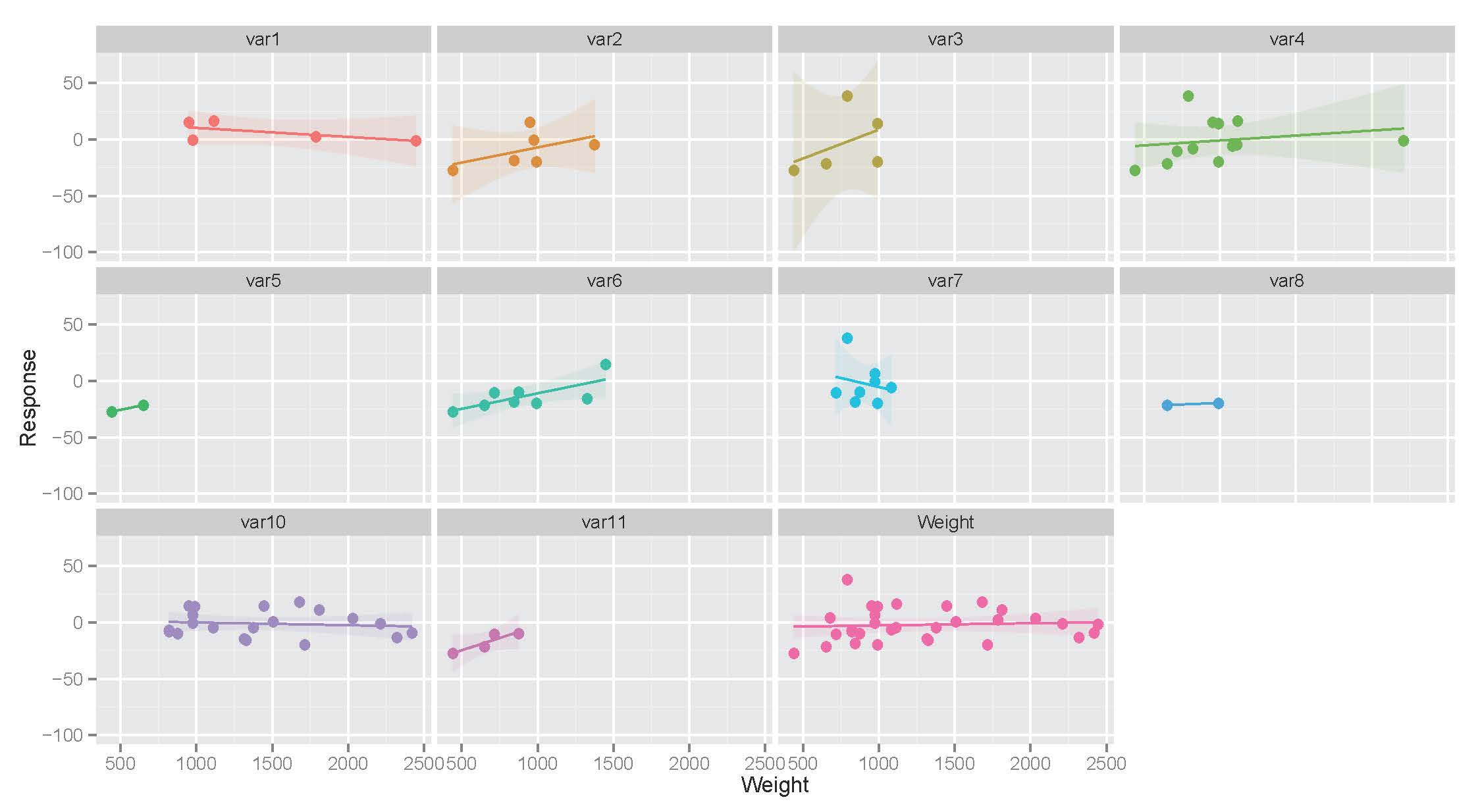
To help visualize the data, and the effect of Weight on the Response, I've constructed the follow plots. In the second plot, I attempt to control for the natural Response~Weight relationship.
 #GRAPH
 library(ggplot2)
 library(reshape2)

 Data <- read.table("Fake Data.txt",header=TRUE)
 #Creating long format for ggplot2
 Data2<-melt(Data, id.vars = c("Subject","Response","Weight"), measure.vars = c("var1","var2","var3","var4","var5","var6","var7","var8","var10","var11"))

 #Adding in weight to the varibles to be plotted
 Data2<-rbind(Data2,Data2[1:31,])
 levels(Data2$variable)<-c(levels(Data2$variable),"Weight")
 Data2[311:341,4]<-"Weight"
 Data2[311:341,5]<-1

 #Removing rows where the categorical variable is 0=No
 for(i in 1:length(Data2[,1])){
 if(Data2[i,5]==0)Data2[i,]<-NA
 }
 Data3<-na.omit(Data2)

 #Plotting Response vs Weight for each 'Yes' group for the categorical variables
  scatter <- ggplot(Data3, aes(Weight, Response, colour = variable))
 scatter + geom_point(aes(color = variable), size = 3) + geom_smooth(method = "lm",aes(fill = variable), alpha = 0.1) + facet_wrap(~variable)+ guides(fill=FALSE,color=FALSE)

 #Zeroing the Response~Weight relationship to remove its influence. Correction coefficients from linear model fit to Response~Weight
 Data4<-Data3
 Data4$Response<-Data4$Response-(0.01494*(Data4$Weight)+ 84.67715)

 #Plotting Response vs Weight for each 'Yes' group for the categorical variables for zeroed Response~Weight relationship (as seen in bottom right facet)
 scatter2 <- ggplot(Data4, aes(Weight, Response, colour = variable))
 scatter2 + geom_point(aes(color = variable), size = 3) + geom_smooth(method = "lm",aes(fill = variable), alpha = 0.1) + facet_wrap(~variable)+ guides(fill=FALSE,color=FALSE)

This second plot helps to show how, when the Response~Weight relationship is controlled for, variables like 'var10' have no influence on the response, while variables like 'var11' have all individuals below that zero-centered mean. Thus, from a visual test, I could identify var11 as a categorical variable of interest that negatively influences our response.
Additionally, this plot shows some of the confounding in this dataset, as you can see certain categorical variables 'clump'/are only documented in certain weight ranges. This is due to the underlying biology.
As a final note, I wonder if it is appropriate to use the corrected response in the second plot as the 'Response' for a linear model, thus eliminating the need for a 'Weight' covariate, or if it is incorrect to use such a transformation
Any thoughts are much appreciated
