SVM RBF performance on "dissimilar" data

Question

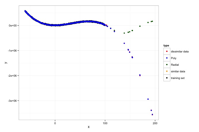
I've been studying the performance of machine learning algorithms on "dissimilar" data (that is, prediction on new data that are not that "similar" to the training set) and I came up with this example where SVM with a radial kernel completely fails, so I would like your opinion on this.

First I generated data from a simple cubic function, but with x restricted from -60 to 100, so the training set starts to show the cubic form but not all of it:

set.seed(100)
f <- function(x) 100*x + 100*x^2 - x^3 + rnorm(length(x), 10000, 10000)
x <- runif(2000, -60, 100)
y <- f(x)

Here is the plot of the training data:

Then I generated additional data of two kinds: (i) similar to the training data (that is, in the range of the observed data); and, (ii) "dissimilar" to the training data (that is, outside of the range of the observed data):

x2 <- runif(20, 60, 200) # dissimilar
y2 <- f(x2)

x3 <- runif(20, -60, 60) # similar 
y3 <- f(x3)

The stripchart of the the data is as follows:

After that I assessed how both the polynomial and the radial kernel SVMs would perform on the dissimilar data set. As expected, the polynomial gets it right, but the radial completely misses it.

svmRadial <- train(as.data.frame(x), y, 
                method = "svmRadial", 
                tuneGrid = expand.grid(.sigma = c(1,5,15,20),
                                       .C = c(0.25, 0.5, 1,4,26,32,64)))

svmPoly <- train(as.data.frame(x), y, method = "svmPoly",
                 tuneGrid = expand.grid(.degree = 1:5,
                                        .scale = c(0.01,0.1, 1),
                                        .C = c(0.25, .5, 1)))

I have played with the tuning parameters, but could not find ones that would make the radial SVM get the pattern right. So:

• Is this a known difficulty with the radial SVM (predicting polynomial patterns out of the predictors range)?

• Could you provide a technical explanation of the hard time SVM is having in this situation?

• Also, if possible, it would be nice to point out some papers on this subject (known limitations of radial kernel SVMs with dissimilar predictors).

Answer 1

Typically, if you have prior knowledge (such as the polynomial form), you should choose your kernel based on that. Secondly, most learning algorithms have problems extrapolating, which is what you are doing. It's more common to look at how well test examples in the same range as the training set are predicted.

Regressing with an RBF kernel is somewhat like doing Fourier analysis (where the spectrum is linked to the kernel bandwidth), as you can see from the nature of the predictions which exhibit some periodicity. Here is an interesting paper on the subject.

I wouldn't consider your observation a limitation in general. You happen to be in a setting which perfectly matches the assumptions of the polynomial kernel, hence it outperforms RBF. This is natural.