A quantitative model emulates some behavior of the world by (a) representing objects by some of their numerical properties and (b) combining those numbers in a definite way to produce numerical outputs that also represent properties of interest.

In this schematic, three numerical inputs on the left are combined to produce one numerical output on the right. The number lines indicate possible values of the inputs and output; the dots show specific values in use. Nowadays digital computers usually perform the calculations, but they are not essential: models have been calculated with pencil-and-paper or by building "analog" devices in wood, metal, and electronic circuits.
As an example, perhaps the preceding model sums its three inputs. R code for this model might look like
inputs <- c(-1.3, 1.2, 0) # Specify inputs (three numbers)
output <- sum(inputs)     # Run the model
print(output)             # Display the output (a number)
Its output simply is a number,
-0.1
We cannot know the world perfectly: even if the model happens to work exactly the way the world does, our information is imperfect and things in the world vary. (Stochastic) simulations help us understand how such uncertainty and variation in the model inputs ought to translate into uncertainty and variation in the outputs. They do so by varying the inputs randomly, running the model for each variation, and summarizing the collective output.
"Randomly" does not mean arbitrarily. The modeler must specify (whether knowingly or not, whether explicitly or implicitly) the intended frequencies of all the inputs. The frequencies of the outputs provide the most detailed summary of the results.

The same model, shown with random inputs and the resulting (computed) random output.
The figure displays frequencies with histograms to represent distributions of numbers. The intended input frequencies are shown for the inputs at left, while the computed output frequency, obtained by running the model many times, is shown at right.
Each set of inputs to a deterministic model produces a predictable numeric output. When the model is used in a stochastic simulation, however, the output is a distribution (such as the long gray one shown at right). The spread of the output distribution tells us how the model outputs can be expected to vary when its inputs vary.
The preceding code example might be modified like this to turn it into a simulation:
n <- 1e5 # Number of iterations
inputs <- rbind(rgamma(n, 3, 3) - 2,
                runif(n, -2, 2),
                rnorm(n, 0, 1/2))
output <- apply(inputs, 2, sum)
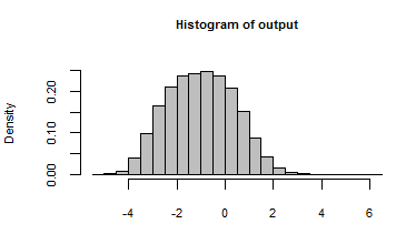
hist(output, freq=FALSE, col="Gray")
Its output has been summarized with a histogram of all the numbers generated by iterating the model with these random inputs:

Peering behind the scenes, we may inspect some of the many random inputs that were passed to this model:
rownames(inputs) <- c("First", "Second", "Third")
print(inputs[, 1:5], digits=2)
The output shows the first five out of $100,000$ iterations, with one column per iteration:
        [,1]  [,2]  [,3]  [,4]  [,5]
First  -1.62 -0.72 -1.11 -1.57 -1.25
Second  0.52  0.67  0.92  1.54  0.24
Third  -0.39  1.45  0.74 -0.48  0.33
Arguably, the answer to the second question is that simulations can be used everywhere. As a practical matter, the expected cost of running the simulation should be less than the likely benefit. What are the benefits of understanding and quantifying variability? There are two primary areas where this is important:
Seeking the truth, as in science and the law. A number by itself is useful, but it is far more useful to know how accurate or certain that number is.
Making decisions, as in business and daily life. Decisions balance risks and benefits. Risks depend on the possibility of bad outcomes. Stochastic simulations help assess that possibility.
Computing systems have become powerful enough to execute realistic, complex models repeatedly. Software has evolved to support generating and summarizing random values quickly and easily (as the second R example shows). These two factors have combined over the last 20 years (and more) to the point where simulation is routine. What remains is to help people (1) specify appropriate distributions of inputs and (2) understand the distribution of outputs. That is the domain of human thought, where computers so far have been little help.


