How to simplify a stretched exponential fit?

Question

I have data from a Monte Carlo experiment that I was hoping to fit to a model of the form $$\log(x y) \approx \beta_0 + \beta_1 \log(z),$$ where I have many observations of triplets, $x, y, z$. This fit does a decent job, but when I look at the residuals of the fit versus $\log(z)$, there is a tell-tale bowl shape:

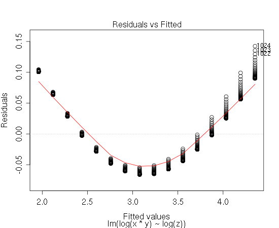
This suggests a fit of the form $$\log(x y) \approx \beta_0 + \beta_1 \log(z) + \beta_2 \left(\log(z)\right)^2,$$ I am not entirely opposed to such a fit, but my final goal is to state an equation that gives $x$ concisely in terms of $y$ and $z$. When I take the exponent of both sides of this fit, I get something really ugly: $$x = \frac{c_0 z^{c_1 + c_2 \log(z)}}{y}$$ This was not what I was hoping for.

Is there some trick that I can use to get out of this mess? Ideally I would have one less constant, or at least not have a $z^{\log{z}}$ term.

edit: There is a strong theoretical reason to favor a fit of this form, instead of putting $\log y$ on the right hand side and performing a 'full' fit. If you do that, the coefficient associated with $\log y$ is nearly -1 anyway (-0.9989), but if you do, you do not see this 'quadratic' artifact with respect to the fitted values. It turns out that the $z=1$ case is a well known phenomenon for which $x = c / y$ is the commonly accepted law.

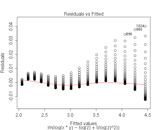
If it helps any, when I plot the residuals versus the more general model $$\log(x y) \approx \beta_0 + \beta_1 \log(z) + \beta_2 \left(\log(z)\right)^2,$$ I get this:

Answer 1

The first thing to do, if possible, is to take care of the heteroscedasticity. Notice how the spread of the residuals consistently increases with the fit: in fact, the spread seems to increase almost quadratically with larger fit.

A standard cure is to return to the original response ($log(xy)$) and apply a strong transformation, such as a logarithm or even a reciprocal: something in that range is suggested by this pattern of heteroscedasticity. Then redo the fitting and recheck the residuals.

It's a good idea to fit lines by eye, using graphs of transformed $xy$ against $z$ (or $\log(z)$. This usually reveals more than any amount of manipulating a regression routine. Once you have a suitable model, you can finally use least squares (or robust regression) to produce a final fit.

In this instance you might also want to explore the relationships among $x$ and $z$ and $y$ and $z$ separately to see whether just one of $x$, $y$ is causing the sudden change in slope between 2.9 and 3.6. The change clearly is not quadratic: both "limbs" of the residual plot are linear. One way to model this change--if it persists after you have dealt with the heteroscedasticity--is with a changepoint model that posits one value of the slope $\beta_1$ for, say, $z \le 3.2$, and a different value for $z \gt 3.2$.

Finally, in Monte-Carlo simulations you have full control and you know exactly the mechanism that produces the responses. It can be useful to subject this to some analysis to find out just what the correct relationship among the triples ought to be.