Interpretation of interaction between a PC and a continuous predictor on a logical response

Question

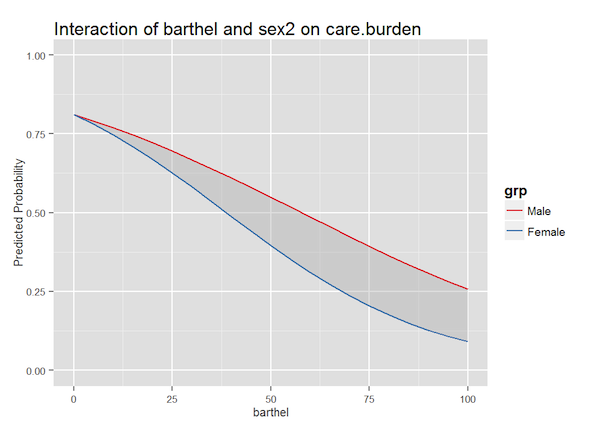
I'm using lme4 in R to test the effect of various continuous explanatory variables, some of which I've corrected for their collinearity using PCA, on a logical response variable.

My optimal model includes a significant interaction between my first principal component and a predictor variable (external to the PCs) which has a positive regression coefficient. I'm not quite sure how to interpret this two-way interaction. Does Fs_abundance increase with an unit increase of the positive loadings and decrease of negative loadings of PC1 and that increases the likelihood of success of my response variable?

a12 <- glmer(Tb_qpcr_status ~ (1|River) + Fs_abundance * PC1, 
family = binomial, data = f.data)

summary(a12)

Generalized linear mixed model fit by maximum likelihood (Laplace Approximation) ['glmerMod']
 Family: binomial  ( logit )
Formula: Tb_qpcr_status ~ (1 | River) + Fs_abundance * PC1
   Data: f.data

     AIC      BIC   logLik deviance df.resid 
    16.7     19.9     -3.4      6.7        9 

Scaled residuals: 
    Min      1Q  Median      3Q     Max 
-1.1975 -0.1143 -0.0185  0.1221  1.4067 

Random effects:
 Groups Name        Variance Std.Dev.
 River  (Intercept) 0        0       
Number of obs: 14, groups:  River, 3

Fixed effects:
                 Estimate Std. Error z value Pr(>|z|)
(Intercept)       -4.6814     3.9753  -1.178    0.239
Fs_abundance       2.1215     2.8837   0.736    0.462
PC1               -0.9542     1.7018  -0.561    0.575
Fs_abundance:PC1   3.5402     2.7761   1.275    0.202

Correlation of Fixed Effects:
            (Intr) Fs_bnd PC1   
Fs_abundanc -0.713              
PC1          0.759 -0.758       
Fs_bndn:PC1 -0.684  0.427 -0.123  

---

a13 <- update(a12, ~.- Fs_abundance:PC1)
anova(a12, a13)

Data: f.data
Models:
a13: Tb_qpcr_status ~ (1 | River) + Fs_abundance + PC1
a12: Tb_qpcr_status ~ (1 | River) + Fs_abundance * PC1
    Df    AIC    BIC  logLik deviance  Chisq Chi Df Pr(>Chisq)  
a13  4 19.640 22.197 -5.8201   11.640                           
a12  5 16.721 19.916 -3.3605    6.721 4.9192      1    0.02656 *
---
Signif. codes:  0 ‘***’ 0.001 ‘**’ 0.01 ‘*’ 0.05 ‘.’ 0.1 ‘ ’ 1

Answer 1

To understand interactions in logistic regression, I found this posting helpful.

I personally find visual inspection helpful, especially when you have interaction terms in logistic regression. In my sjPlot-package there's a function to plot interaction terms of (generalized) linear (mixed effects) models. You can find some examples in this online-manual. The formula to calculate the interaction is based on what Karen Grace described here and here.

For logistic regressions, the odds ratios are translated into probabilities.

Here's an example from the sample data set with a simple glm:

# load sample data
data(efc)
# create binary response
care.burden <- ifelse(efc$neg_c_7 < median(na.omit(efc$neg_c_7)), 0, 1)
# create data frame for fitted model
mydf <- data.frame(care.burden = as.factor(care.burden),
                   sex = as.factor(efc$c161sex),
                   barthel = as.numeric(efc$barthtot))
# fit model
fit <- glm(care.burden ~ sex * barthel,
           data = mydf,
           family = binomial(link = "logit"),
           x = TRUE)
# plot interaction, increase p-level sensivity
sjp.int(fit,
        legendLabels = get_val_labels(efc$c161sex),
        plevel = 0.1)