Including random terms in the model is a way to induce some covariance structure bteween the grades. The random factor for the school induces a non zero covariance between different students from the same school, whereas it is $0$ when the school are different.
Let's write your model as
$$ Y_{s,i} = \alpha + \text{hours}_{s,i} \beta + \text{school}_s + e_{s, i} $$
where $s$ indexes the school and $i$ indexes the students (in each school). The terms $\text{school}_s$ are independent random variables drawn in a $\mathcal N(0, \tau)$. The $e_{s, i}$ are independent random variables drawn in a $\mathcal N(0, \sigma^2)$.
This vector has expected value
$$\left[ \alpha + \text{hours}_{s,i} \beta \right]_{s,i}$$
which is determined by the number of worked hours.
The covariance between $Y_{s,i}$ and $Y_{s',i'}$ is $0$ when $s \ne s'$, which means that the departure of the grades from the expected values are independent when the students are not in the same school.
The covariance between $Y_{s,i}$ and $Y_{s,i'}$ is $\tau$ when $i \ne i'$, and the variance of $Y_{s,i}$ is $\tau + \sigma^2$: grades of students from the same school will have correlated departures from their expected values.
Example and simulated data
Here is a short R simulation for fifty students from five schools (here I take $\sigma^2 = \tau = 1$); the names of the variable are self documenting:
set.seed(1)
school        <- rep(1:5, each=10)
school_effect <- rnorm(5)

school_effect_by_ind <- rep(school_effect, each=10)
individual_effect    <- rnorm(50)
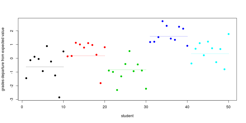
We plot the departures from expected grade for each student, that is the terms $\text{school}_s + e_{s, i}$, together with (dotted line) the mean departure for each school:
plot(individual_effect + school_effect_by_ind, col=school, pch=19,
     xlab="student", ylab="grades departure from expected value")
segments(seq(1,length=5,by=10), school_effect, seq(10,length=5,by=10), col=1:5, lty=3)

Now let's comment on this plot. The level of each dotted line (corresponding to $\text{school}_s$) is drawn at random in a normal law. The student specific random terms are also drawn at random in a normal law, they correspond to the distance of the points from the dotted line. The resulting value is, for each student, the departure from $\alpha + \text{hours} \beta$, the grade determined by the time spent to work. As a result, pupils in the same school are more similar to each other than pupils from different schools, as you stated in your question.
The variance matrix for this example
In the above simulations we draw separately the school effects $\text{school}_s$ and the individual effects $e_{s,i}$, so the covariance considerations with which I began don’t appear clearly here. In fact, we would have obtained similar results by drawing a random normal vector of dimension 50 with block-diagonal covariance matrix
$$\left[\begin{matrix}
A & 0 & 0 & 0 & 0 \\
0 & A & 0 & 0 & 0 \\
0 & 0 & A & 0 & 0 \\
0 & 0 & 0 & A & 0 \\
0 & 0 & 0 & 0 & A
\end{matrix}\right]$$
where each of the five $10\times 10$ blocks $A$ correspond to the covariance between the students of a same school:
$$A = \left[\begin{matrix}
2 & 1 & 1 & 1 & 1 & 1 & 1 & 1 & 1 & 1\\
1 & 2 & 1 & 1 & 1 & 1 & 1 & 1 & 1 & 1\\
1 & 1 & 2 & 1 & 1 & 1 & 1 & 1 & 1 & 1\\
1 & 1 & 1 & 2 & 1 & 1 & 1 & 1 & 1 & 1\\
1 & 1 & 1 & 1 & 2 & 1 & 1 & 1 & 1 & 1\\
1 & 1 & 1 & 1 & 1 & 2 & 1 & 1 & 1 & 1\\
1 & 1 & 1 & 1 & 1 & 1 & 2 & 1 & 1 & 1\\
1 & 1 & 1 & 1 & 1 & 1 & 1 & 2 & 1 & 1\\
1 & 1 & 1 & 1 & 1 & 1 & 1 & 1 & 2 & 1\\
1 & 1 & 1 & 1 & 1 & 1 & 1 & 1 & 1 & 2
\end{matrix}\right].$$

