Power of a case control test as a function of $P(X=1)$ & $P(Y=1)$

Question

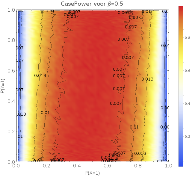
For our course in statistics we had to build a simulation which would give insight in the power of a case-control study vs that of a cohort study, both trying to discover an association between 2 binary variables ($X$ and $Y$).
To determine wether $X$ and $Y$ were associated the tests calculated the odds-ratio of a sample and used the central limit theorem to calculate a $97.5$% confidence interval.
The tests were one-sided as we assumed an odds-ratio higher than $1$.
The power was calculated by performing multiple tests and taking the mean of the amount of times the null-hypothesis (no association) was rejected.

This was done for multiple populations, each with $P(X=1)$ and $P(Y=1)$ in the range $[0,1]$.

The strange thing is that when we plotted the power as a function of $P(X=1)$ and $P(Y=1)$ we got:

(the contours denote the estimated std on the power, the image was smoothened by using spline interpolation, about 10000 datapoints were used neatly spread over the plane)

Which is not really what you would expect: there seems to be some dependency on $P(Y=1)$, even though the whole idea of an idealised (which it is due the simulation) case-control studie is that it should not depend on $P(Y=1)$. We showed the result to our professor and he seemed puzzled too by this result.

How we got the exact result:

1. We chose an odds-ratio $OR$

2. we let $P(Y=1)=\mathrm{L}(\alpha+X\beta)$ (with $\mathrm L$ the logistic function), $\beta=\ln(OR)$, $\alpha$ a parameter describing external effects.

3. we let $P(X=1$ range from $0$ to $1$ in about $50$ steps

4. we let $\alpha$ (and thus $P(Y=1)$) range from $-10$ to $10$ in about $200$ steps

5. we took $1000$ case-control samples and calculated the $OR$ and CI by using the central limit theorem

6. by taking the mean of the amount of rejections of the null-hypothesis we determined the power of the test

The R-code we used to calculate the data was the following:

npop    <- 10000000                # Population size
nsample <- 1000                    # Sample size
nsim    <- 1000                    # Amount of simulations
pvals   <- seq(0.01,0.99,0.98/50)  # P(X=1)
alphas  <- seq(-10,10,0.1)         # Needed to calculate P(Y=1)

mat             <- matrix(NA, nrow = length(alphas)*length(pvals), 
                          ncol = 5)
colnames(mat)   <- c("PX1", "PY1", "CasePower", "CaseStd")

### Functions
# To estimate the std we use the jackknife
jackknife <- function(vec){
    l <- length(vec)
    power <- mean(vec, na.rm=TRUE)
    pseudov <- c()
    
    for (i in 1:l){
        pseudov[i] <- l*power - (l-1)*mean(vec[-i], na.rm=TRUE)
    }
    sqrt(var(pseudov, na.rm=TRUE)/l)
}

# Calculate whether to reject the null hypothesis or not (based on 
# calculating the odds-ratio)
ORatio <- function(vec){
    n00 <- vec[4]  #= number of cases where x = 0 and y = 0
    n01 <- vec[3]  #= number of cases where x = 0 and y = 1
    n10 <- vec[2]  #= number of cases where x = 1 and y = 0
    n11 <- vec[1]  #= number of cases where x = 1 and y = 1
    
    OR <- (n00/n10) * (n11/n01)                           
    siglog <- sqrt((1/n00) + (1/n01) + (1/n10) + (1/n11)) 
    zalph <- qnorm(1 - 0.05/2)                            
    
    orlo <- OR/(exp(zalph*siglog))                        
    
    if(is.nan(orlo) || is.na(orlo)){                      
        NaN
    }else{
        if(orlo<1){                                       
            0
        }else{                                            
            1
        }
    }
}

# The simulation
    for(p in 1:length(pvals)){
        pval <- pvals[p]
        for(a in 1:length(alphas)){
            alpha  <- alphas[a]
            A      <- 1/(exp(-alpha)+1)
            B      <- 1/(exp(-alpha-beta)+1)
            qval   <- (1-pval)*A + pval*B      # P(Y=1)
            
  # If the values of P(Y=1) or P(X=1) are too extreme they'll only 
  # result in NA's so we better refuse to use them now
            if(qval>0.005 && qval<0.995){
            counter = counter + 1
            
     # First two columns of 'mat' are filled with P(X=1) and P(Y=1)
            data[[b]][counter,1] <- pval    # P(X=1)
            data[[b]][counter,2] <- qval    # P(Y=1)
            
            # Simulate the population
            # 4 columns: x & y, x & ~y, ~x & y, ~x & ~y
            population  <- rmultinom(1, npop, c(B*pval, pval*(1-B), 
                             A*(1-pval), (1-A)*(1-pval)))[,1]
                          
            # [[ CASE ]] 
            list1      <- rbinom(nsim, nsample/2, population[1]/
                    (population[1] + population[3]))
            list2      <- rbinom(nsim, nsample/2, population[2]/
                    (population[2] + population[4]))
            list3      <- nsteek/2 - list1
            list4      <- nsteek/2 - list2
            
            results    <- rbind(list1, list2, list3, list4)
            succesList <- apply(results, 2, ORatio)
            Casepower  <- mean(succesList, na.rm = TRUE)
            CaseStd    <- jackknife(succesList)
            
            # Add the data to 'mat'
            data[[b]][counter,3] <- Casepower
            data[[b]][counter,4] <- CaseStd
            }
        }
    }
}

If anyone would have an idea why we observe this small dependency on $P(Y=1)$ and would like to share it, it would be greatly appreciated.

Answer 1

Ok, so you probably don't care about this any more since it's been nine years, but it's an interesting question. What I think is going on is that the joint distribution of $X$ and $Y$ changes in the sample because the odds ratio is not 1.

When $P(Y=1)=0.5$ the power seems to be maximised at $P(X=1)=0.5$, which makes sense from symmetry. When $P(Y=1)>0.5$ the power is maximised at $P(X=1)>0.5$ and vice versa.

Thinking about this, suppose that $P(Y=1)$ is small (the usual case-control setting). Then $P(X=1)$ in the sample is larger than $P(X=1)$ in the population, because cases are more likely than controls to be exposed. If $P(X=1)=0.5$ in the population then $P(X=1)>0.5$ in the sample. Reducing $P(X=1)$ in the population will lead to slightly higher power.

Conversely, suppose that $P(Y=1)$ is large. Then $P(X=1)$ in the sample is smaller than $P(X=1)$ in the population, because we are subsampling cases, and cases are more likely than controls to be exposed. If $P(X=1)=0.5$ in the population then $P(X=1)<0.5$ in the sample. Increasing $P(X=1)$ in the population will lead to slightly higher power.