6
$\begingroup$

I have a data set that looks like the following:

dates, product, salesman, sales
2015-05-01, Product1, Salesman1, 100
2015-05-01, Product1, Salesman2, 300
2015-05-01, Product1, Salesman3, 400
2015-05-01, Product1, Salesman4, 120
2015-05-01, Product1, Salesman5, 290
2015-05-01, Product1, Salesman6, 210
2015-05-01, Product2, Salesman1, 500
2015-05-01, Product2, Salesman2, 90
2015-05-01, Product2, Salesman3, 100
2015-05-01, Product2, Salesman4, 50
2015-05-01, Product2, Salesman5, 320
2015-05-01, Product2, Salesman6, 120
2015-05-09, Product1, Salesman1, 10
2015-05-09, Product1, Salesman2, 200
2015-05-09, Product1, Salesman3, 400
2015-05-09, Product2, Salesman1, 200
2015-05-09, Product2, Salesman2, 40
2015-05-09, Product2, Salesman3, 10
2015-05-09, Product2, Salesman4, 120
2015-05-09, Product2, Salesman5, 20
2015-05-09, Product2, Salesman6, 500
2015-05-20, Product1, Salesman1, 100
2015-05-20, Product1, Salesman2, 300
2015-05-20, Product1, Salesman3, 400
2015-05-20, Product2, Salesman1, 200
2015-05-20, Product2, Salesman2, 180
2015-05-20, Product2, Salesman3, 20
2015-05-20, Product2, Salesman4, 20
2015-05-20, Product2, Salesman5, 40
2015-05-20, Product2, Salesman6, 40

And I need to visualise this effectively. Currently, I am using the following visualisation (visualisation code along with data generation)

df1 <- read.csv(header = TRUE, text = 
    "dates, product, salesman, sales
    2015-05-01, Product1, Salesman1, 100
    2015-05-01, Product1, Salesman2, 300
    2015-05-01, Product1, Salesman3, 400
    2015-05-01, Product1, Salesman4, 120
    2015-05-01, Product1, Salesman5, 290
    2015-05-01, Product1, Salesman6, 210
    2015-05-01, Product2, Salesman1, 500
    2015-05-01, Product2, Salesman2, 90
    2015-05-01, Product2, Salesman3, 100
    2015-05-01, Product2, Salesman4, 50
    2015-05-01, Product2, Salesman5, 320
    2015-05-01, Product2, Salesman6, 120
    2015-05-09, Product1, Salesman1, 10
    2015-05-09, Product1, Salesman2, 200
    2015-05-09, Product1, Salesman3, 400
    2015-05-09, Product2, Salesman1, 200
    2015-05-09, Product2, Salesman2, 40
    2015-05-09, Product2, Salesman3, 10
    2015-05-09, Product2, Salesman4, 120
    2015-05-09, Product2, Salesman5, 20
    2015-05-09, Product2, Salesman6, 500
    2015-05-20, Product1, Salesman1, 100
    2015-05-20, Product1, Salesman2, 300
    2015-05-20, Product1, Salesman3, 400
    2015-05-20, Product2, Salesman1, 200
    2015-05-20, Product2, Salesman2, 180
    2015-05-20, Product2, Salesman3, 20
    2015-05-20, Product2, Salesman4, 20
    2015-05-20, Product2, Salesman5, 40
    2015-05-20, Product2, Salesman6, 40")


levels(df1$dates) <- c('2015-05-01', '2015-05-09', '2015-05-20', '2015-05-01')

library(ggplot2)
library(magrittr)


df1 %>% ggplot(aes(x = dates, y = salesman)) + geom_tile(aes(fill = sales), colour = 'white') + scale_fill_gradient(low = 'white', high = 'steelblue') + theme_bw() + theme
(panel.grid = element_blank(), panel.border = element_blank()) + facet_grid(product ~ ., scales = 'free')
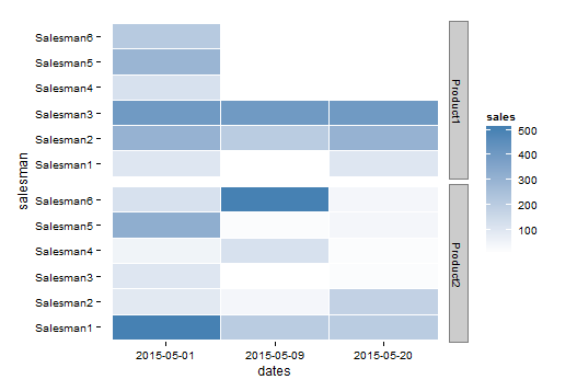
enter image description here

My objective is to show how each salesman's performance was during the recorded days, for each of the product types. I want to facilitate comparison of each salesman's current and old performance, so I have used dates on x-axis to enable easy comparison. I also want to compare the performance intra-products and inter-products, so I have used facets from ggplot2.

My reservation on using a line/bar chart was that if more salesmen are added to the data set, it will quickly become difficult to compare each salesman to the other. Plus, it will also be difficult to compare performance across the recorded dates.

The audience are business managers who are only moderately literate about Statistics.They are not used to seeing box plots, heatmaps, but are open to them nonetheless. They have primarily seen the humble bar and line charts, using only the basic scales, rather than logarithmic scales.

Questions:

  • Would you suggest any alternative visualisation for such data - I understand some people may find it difficult to perceive trends if they are shown using colours, so there must be a better alternative?
  • If I stick to the current visualisation, should data labels also be added to show what value for sales is for each salesman? I do think that it clutters the visualisation.

PS. Although I am using ggplot2 in R, and would appreciate any R solutions, I am really after a visualisation, regardless of the software/code used to produce it, and for the latter I will be especially thankful.

$\endgroup$
7
  • 1
    $\begingroup$ Can you post your plot here? $\endgroup$
    – rnso
    Commented May 29, 2015 at 13:19
  • 1
    $\begingroup$ It is important to post a plot, for otherwise this question really isn't intelligible without requiring readers to run your code. Also consider explaining the purpose of the visualization as well as giving the characteristics of the intended audience. $\endgroup$
    – whuber
    Commented May 29, 2015 at 13:30
  • 3
    $\begingroup$ Be careful of making your Q seem too R specific. I think it is fine to say that you are using R & that R-based solutions would be especially helpful, but note that asking for R code per se is off-topic here. Also, some of our most prolific [data-visualization] experts / answerers here use software other than R, & you wouldn't want to preclude their insights. $\endgroup$ Commented May 29, 2015 at 15:28
  • 1
    $\begingroup$ I don't think your Q, as stated, is necessarily too R specific, but the phrasing "Using ggplot2,", is on the borderline. $\endgroup$ Commented May 29, 2015 at 15:35
  • 1
    $\begingroup$ +1 This has turned into a very well-formulated question, thank you. $\endgroup$
    – whuber
    Commented May 29, 2015 at 17:03

2 Answers 2

4
$\begingroup$

A tangent suggestion since this thread has come to the top... Ordering groups alphabetically is rarely meaningful for plotting. If a better ordering doesn't exist, as may be the case for names of salesmen, you can hierarchically cluster the salesmen and use the ladderized dendrogram to bring similar salesmen close to each other in the plot panels. (It sounds quite messy and complex but it's not that bad and I had good results with gene expression data.)

It works nicely when you have more than a few groups so for the sake of example I'm going to duplicate the OP's dataset to have 12 salesmen:

library(data.table)
library(ggplot2)
library(dendextend)

set.seed(1234)

df1<-read.csv(header=TRUE,text=
    "dates,product,salesman,sales
    2015-05-01,Product1,Salesman1,100
    2015-05-01,Product1,Salesman2,300
    2015-05-01,Product1,Salesman3,400
    2015-05-01,Product1,Salesman4,120
    2015-05-01,Product1,Salesman5,290
    2015-05-01,Product1,Salesman6,210
    2015-05-01,Product2,Salesman1,500
    2015-05-01,Product2,Salesman2,90
    2015-05-01,Product2,Salesman3,100
    2015-05-01,Product2,Salesman4,50
    2015-05-01,Product2,Salesman5,320
    2015-05-01,Product2,Salesman6,120
    2015-05-09,Product1,Salesman1,10
    2015-05-09,Product1,Salesman2,200
    2015-05-09,Product1,Salesman3,400
    2015-05-09,Product2,Salesman1,200
    2015-05-09,Product2,Salesman2,40
    2015-05-09,Product2,Salesman3,10
    2015-05-09,Product2,Salesman4,120
    2015-05-09,Product2,Salesman5,20
    2015-05-09,Product2,Salesman6,500
    2015-05-20,Product1,Salesman1,100
    2015-05-20,Product1,Salesman2,300
    2015-05-20,Product1,Salesman3,400
    2015-05-20,Product2,Salesman1,200
    2015-05-20,Product2,Salesman2,180
    2015-05-20,Product2,Salesman3,20
    2015-05-20,Product2,Salesman4,20
    2015-05-20,Product2,Salesman5,40
    2015-05-20,Product2,Salesman6,40")
df1<-as.data.table(df1)
levels(df1$dates) <- c('2015-05-01', '2015-05-09', '2015-05-20')
df2 <- copy(df1)
df2[, salesman := sprintf('A%s', salesman)]
df2[, sales := rpois(n=length(sales), sales * 1.2)]
df1 <- rbind(df1, df2)

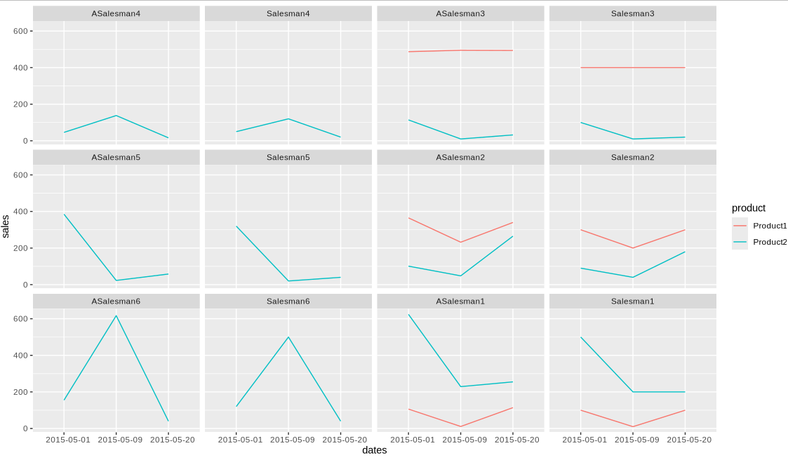
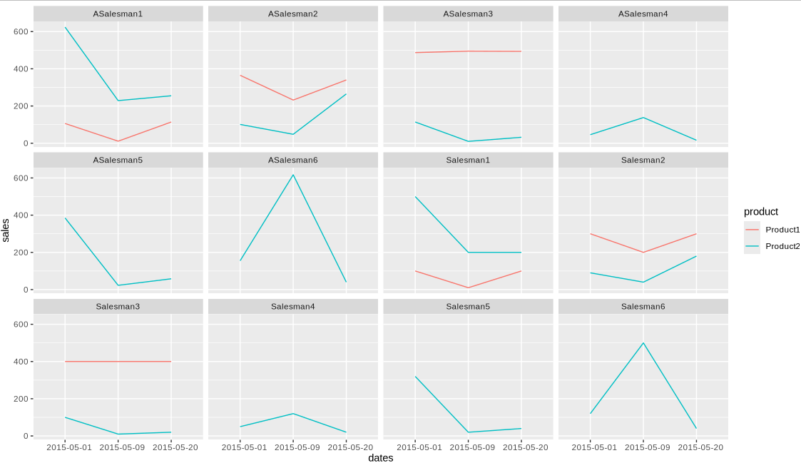
Alphabetical ordering makes it difficult to notice for example that "A Salesman 4" is similar to "Salesman 4":

gg <- ggplot(data=df1, aes(x=dates, y=sales, group=product, colour=product)) +
    geom_line() +
    facet_wrap(~salesman, ncol=4)

enter image description here

However, after clustering and reordering some similarities become clear:

mat <- dcast(salesman ~ dates, value.var='sales', data=df1[product == 'Product2'])
mat <- scale(as.matrix(mat, rownames='salesman'))
hc <- ladderize(as.dendrogram(hclust(dist(mat))))
df1[, salesman2 := factor(salesman, labels(hc))]

gg <- ggplot(data=df1, aes(x=dates, y=sales, group=product, colour=product)) +
    geom_line() +
    facet_wrap(~salesman2, ncol=4)

"A Salesman4" is next to "Salesman4" and "3" is closer to "5" (since I clustered on Product2)

enter image description here


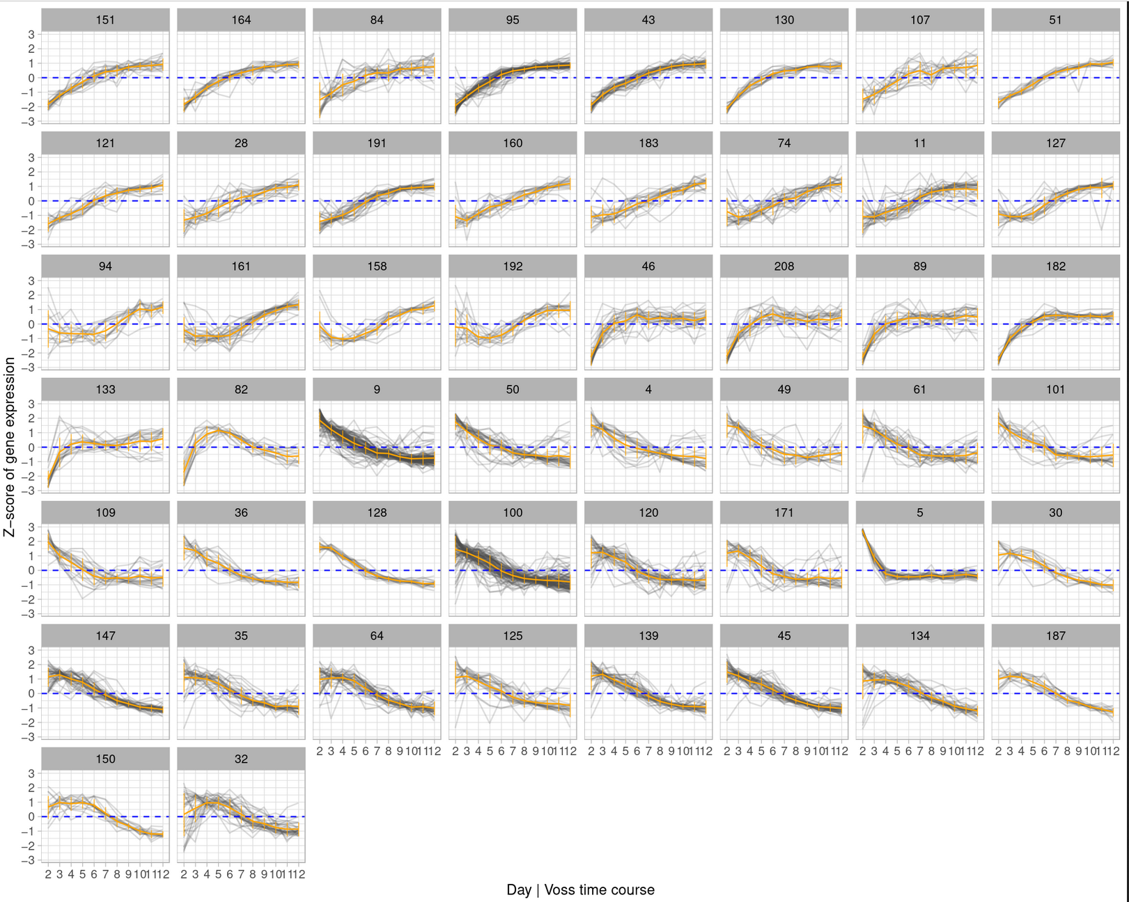
EDIT: This below is an example where I was quite pleased with the ordering by clusters. Panels names are just identifiers with no intrinsic meaning.

enter image description here

$\endgroup$
2
  • 4
    $\begingroup$ This is a good point not just here but more generally. Alphabetical order is often far from ideal for seeing structure. Howard Wainer has mocked it as "Alabama first" or "Austria first" to which can be added easily "Aberdeen first". But conversely while clustering may help, or even be necessary, it is more common in my experience that something really simple like sorting on series mean or the last value is fine. Once the point is seen it doesn't need much expansion, but there are some general comments and more examples within journals.sagepub.com/doi/pdf/10.1177/1536867X211045582 $\endgroup$
    – Nick Cox
    Commented May 3 at 12:15
  • 3
    $\begingroup$ For Wainer see e.g. jstor.org/stable/2683253 $\endgroup$
    – Nick Cox
    Commented May 3 at 12:18
3
$\begingroup$

Your visualization duplicates the "salesman" rows, which worsens the problem relative to adding more salespeople.

In addition, if you use color to show quantity, absence of data could be mistaken for 0 (unless you choose different colors for 0 and for missing data, and make it very explicit in the legend, but it may require additional cognitive processing for your audience). It could be important to make the distinction between the two, e.g. it could be very well that the salespeople did sell products, but the system had a bug that prevented data entry at some point.

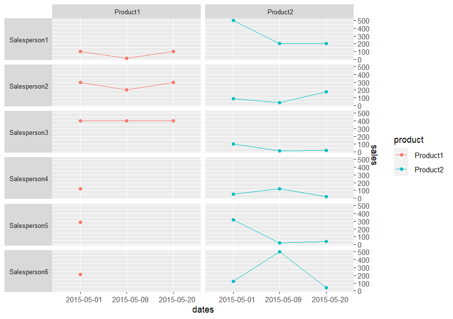
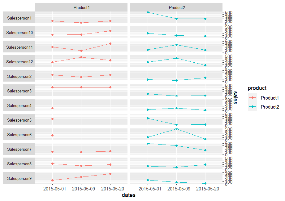
Small multiple (or facet grid) with a series of line charts could work, with "salesperson" as main rows and "product" as main columns, and within each cell "dates" as the x axis and "sales" as the y axis. It allows comparison between products and between salespeople, doesn't have the problem of duplicated rows that your original attempt had, and you immediately spot missing data:

Small multiple of line charts. Main rows consist of each salesperson, main columns consist of products, and cells are line charts with dates on the x axis, and number of cells on the y axis. It appears that some salespeople have missing data for some dates.

Using lines combined with points allows a more specific identification of the missing data problem. Using only lines without points would generate completely empty graphs for the cells in question, so you wouldn't see for which specific dates data is missing.

The legend is redundant with the columns, but this is not necessarily an issue, as redundant information can allow a more efficient extraction of information. Testing it on a couple of "naive" test subjects before showing it to a larger audience could be a good idea, to check if the redundant legend could create confusion for your intended audience, or if on the contrary it is helpful.

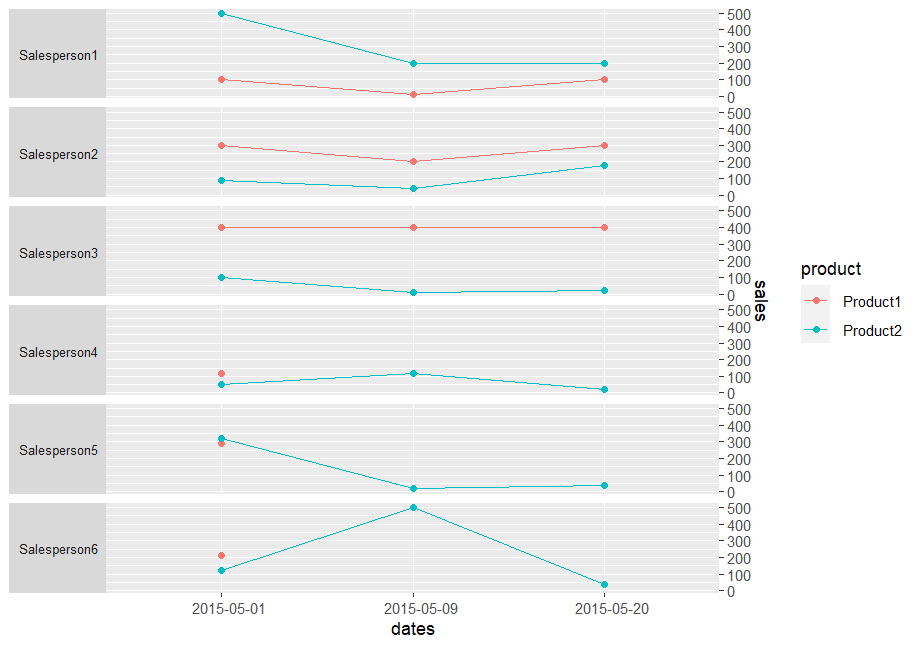
You could combine the "product" columns into a single column, so each cell would consist of two lines instead of a single one. However, after a couple of tests, I find that the graph feels more cluttered this way, even if I'm not entirely sure why (maybe because it makes it a bit more difficult to distinguish which 'product' line belongs to which salesperson):

Attempt of a small multiple similar to the previous one, except that there's a single column, and each cell consists of a line chart with two lines: one for "product1", and a second one for "product2".

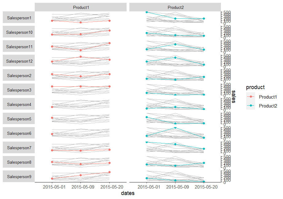
If you want to include more salespeople and want to be able to compare salespeople between them, you could plot greyed out lines of all salespeople in each cell (with the overlaid colored line of the salesperson corresponding to the row). This is far from being a perfect solution, though. Here's an example, with 12 salespeople:

Graph similar to the first one, except there are 12 salespeople, and each cells also contain greyed out lines of the sales of all other salespeople for the product.

A problem is that you have to specify to your audience what the grey lines represent exactly. For instance in column "product1", they are the lines of all salespeople for product1, not for all products. Without specifying it explicitly, it may require a non-trivial effort for your audience to find out what these grey lines represent - assuming this is even possible to find out in the first place.

In addition, I find it feels somehow cluttered (and I didn't correct the overlapping values on the y axis on the right, which certainly doesn't help). Note that I used a completely white background without grid, because the combo "grid + grey lines" was making my eyes bleed, but of course you could experiment with various grid colors or variants if you find that a grid would make the graph better.

Compare with the same graph without the grey lines (but with a background grid):

Same graph as the previous, without grey lines

Past a certain number of salespeople, I suspect that there would be just too much information to show, and that any kind of visualization would require to use some interactive visualization, or to generate multiple graphs, or to abandon the "salesperson" facet altogether and to regroup them by category (i.e. "salespeople from sector A, B, and C", or whatever classification of interest you may have).


Below is some code in R I used for generating the first visualization from your data. I had to correct the line levels(df1$dates) <- c('2015-05-01', '2015-05-09', '2015-05-20', '2015-05-01'), by removing the last vector element ('2015-05-01') that was a duplicate of the first element. Also, I renamed the variable "salesman" as "Salesperson":

levels(df1$dates) <- c('2015-05-01', '2015-05-09', '2015-05-20')
df1$id2 <- df1$Salesperson
ggplot(df1, aes(x = dates, y = sales, group=product, color=product)) +  
scale_y_continuous(position = "right")+
geom_line(data=df1[,c("dates", "product", "sales", "id2")], aes(x=dates, y=sales, group=id2 ), colour="grey", alpha=0)+
  geom_point() +
  geom_line()+
  facet_grid(Salesperson ~ product, scales = "free", switch="y" )+
  theme(strip.text = element_text(size = 8),strip.text.y.left = element_text(angle = 0))
$\endgroup$
2
  • 2
    $\begingroup$ Excellent advice (+1). Somehow I missed this thread when first posted. Consistent with this, I think, are queries back to the OP. To give even better advice we would need indications: how many sales people, how many products, how many times in the real dataset? What information would you want to emphasise (play down) with a much larger dataset? The dataset here seems fabricated -- reasons why real data are confidential as well as much more extensive are easy to imagine -- but what do the dates mean? Data for intervals of different lengths should be scaled first. $\endgroup$
    – Nick Cox
    Commented May 3 at 8:38
  • 3
    $\begingroup$ (ctd) I agree strongly that heatplots are not a good idea. Sometimes they are the tool of choice, but those I see are usually not nearly as effective as more conventional charts. FYI, the tactic of showing each series in turn with the other series as backdrop has been dubbed front-and-back plots. More important than a name may be some references and further examples. See paper at journals.sagepub.com/doi/pdf/10.1177/1536867X211025838 Since writing that I have found a further informal use of spaghetti for tangled line charts in John Hartigan's 1975 book Clustering Algorithms. $\endgroup$
    – Nick Cox
    Commented May 3 at 8:49

Your Answer

By clicking “Post Your Answer”, you agree to our terms of service and acknowledge you have read our privacy policy.

Not the answer you're looking for? Browse other questions tagged or ask your own question.