Which variable relative importance method to use?

Question

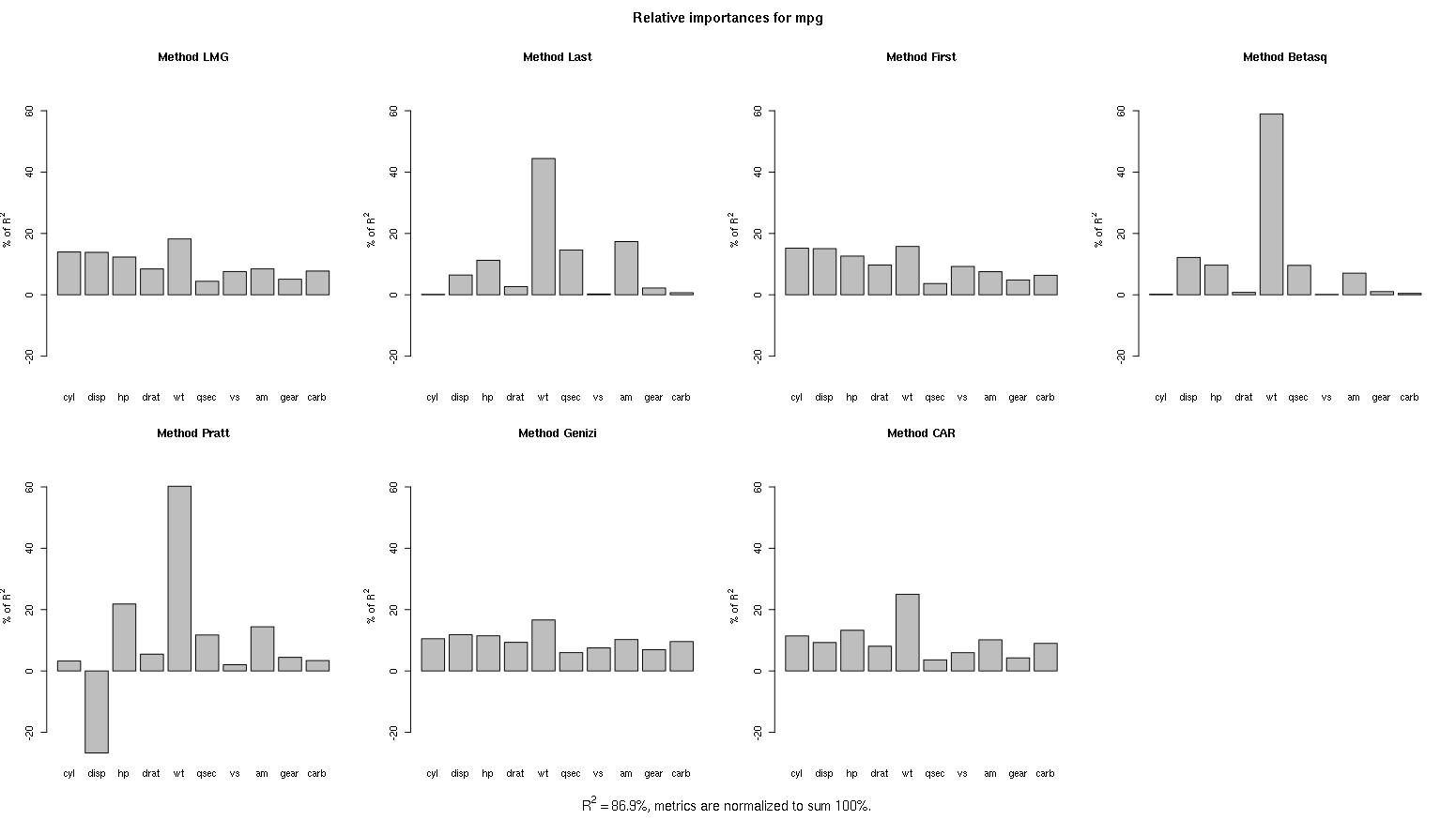
Following is a plot from relaimpo package of R which shows relative importance of predictor variables for regression of mpg on all other variables in mtcars dataset. The relative importance is performed by different methods and the results are quite different. Especially see bars for wt and disp variables. The LMG method is recommended by authors but are there any situation when other methods may be more preferable? Which method would you recommend for general use?

Answer 1

I prefer to compute the proportion of explainable log-likelihood that is explained by each variable. For OLS models the rms package makes this easy:

f <- ols(y ~ x1 + x2 + pol(x3, 2) + rcs(x4, 5) + ...)
plot(anova(f), what='proportion chisq')
# also try what='proportion R2'

The default for plot(anova()) is to display the Wald $\chi^2$ statistic minus its degrees of freedom for assessing the partial effect of each variable. Even though this is not scaled $[0,1]$ it is probably the best method in general because it penalizes a variable requiring a large number of parameters to achieve the $\chi^2$. For example, a categorical predictor with 5 levels will have 4 d.f. and a continuous predictor modeled as a restricted cubic spline function with 5 knots will have 4 d.f.

If a predictor interacts with any other predictor(s), the $\chi^2$ and partial $R^2$ measures combine the appropriate interaction effects with main effects. For example if the model was y ~ pol(age,2) * sex the statistic for sex is the combined effects of sex as a main effect plus the effect modification that sex provides for the age effect. This is an assessment of whether there is a difference between the sexes for any age.

Methods such as random forests, which do not favor additive effects, are not likelihood based, and use multiple trees, require a different notion of variable importance.