24
$\begingroup$

I'm coming from Civil Engineering, in which we use Extreme Value Theory, like GEV distribution to predict the value of certain events, like The biggest wind speed, i.e the value that 98.5% of the wind speed would be lower to.

My question is that why use such an extreme value distribution? Wouldn't it be easier if we just used the overall distribution and get the value for the 98.5% probability?

$\endgroup$

5 Answers 5

30
$\begingroup$

Disclaimer: At points in the following, this GROSSLY presumes that your data is normally distributed. If you are actually engineering anything then talk to a strong stats professional and let that person sign on the line saying what the level will be. Talk to five of them, or 25 of them. This answer is meant for a civil engineering student asking "why" not for an engineering professional asking "how".

I think the question behind the question is "what is the extreme value distribution?". Yes it is some algebra - symbols. So what? right?

Lets think about 1000 year floods. They are big.

When they happen, they are going to kill a lot of people. Lots of bridges are going down.
You know what bridge isn't going down? I do. You don't ... yet.

Question: Which bridge isn't going down in a 1000 year flood?
Answer: The bridge designed to withstand it.

The data you need to do it your way:
So lets say you have 200 years of daily water data. Is the 1000 year flood in there? Not remotely. You have a sample of one tail of the distribution. You don't have the population. If you knew all of the history of floods then you would have the total population of data. Lets think about this. How many years of data do you need to have, how many samples, in order to have at least one value whose likelihood is 1 in 1000? In a perfect world, you would need at least 1000 samples. The real world is messy, so you need more. You start getting 50/50 odds at about 4000 samples. You start getting guaranteed to have more than 1 at around 20,000 samples. Sample doesn't mean "water one second vs. the next" but a measure for each unique source of variation - like year-to-year variation. One measure over one year, along with another measure over another year constitute two samples. If you don't have 4,000 years of good data then you likely don't have an example 1000 year flood in the data. The good thing is - you don't need that much data to get a good result.

Here is how to get better results with less data:
If you look at the annual maxima, you can fit the "extreme value distribution" to the 200 values of year-max-levels and you will have the distribution that contains the 1000 year flood-level. It will be the algebra, not the actual "how big is it". You can use the equation to determine how big the 1000 year flood will be. Then, given that volume of water - you can build your bridge to resist it. Don't shoot for the exact value, shoot for bigger, otherwise you are designing it to fail on the 1000 year flood. If you are bold, then you can use resampling to figure out how much beyond on the exact 1000 year value you need to build it to in order to have it resist.

Here is why EV/GEV are the relevant analytic forms:
The generalized extreme value distribution is about how much the max varies. The variation in the maximum behaves really different than variation in the mean. The normal distribution, via the central limit theorem, describes a lot of "central tendencies".

Procedure:

  1. do the following 1000 times:
    i. pick 1000 numbers from the standard normal distribution
    ii. compute the max of that group of samples and store it
  2. now plot the distribution of the result

    #libraries
    library(ggplot2)
    
    #parameters and pre-declarations
    nrolls <- 1000
    ntimes <- 10000
    store <- vector(length=ntimes)
    
    #main loop
    for (i in 1:ntimes){
    
         #get samples
         y <- rnorm(nrolls,mean=0,sd=1)
    
         #store max
         store[i] <- max(y)
    }
    
    #plot
    ggplot(data=data.frame(store), aes(store)) + 
         geom_histogram(aes(y = ..density..),
                        col="red", 
                        fill="green", 
                        alpha = .2) + 
         geom_density(col=2) + 
         labs(title="Histogram for Max") +
         labs(x="Max", y="Count")
    

This is NOT the "standard normal distribution": enter image description here
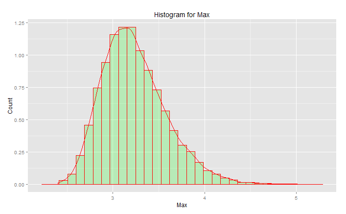
The peak is at 3.2 but the max goes up toward 5.0. It has skew. It doesn't get below about 2.5. If you had actual data (the standard normal) and you just pick the tail, then you are uniformly randomly picking something along this curve. If you get lucky then you are toward the center and not the lower tail. Engineering is about the opposite of luck - it is about achieving consistently the desired results every time. "Random numbers are far too important to leave to chance" (see footnote), especially for an engineer. The analytic function family that best fits this data - the extreme value family of distributions.

Sample fit:
Let's say we have 200 random values of the year-maximum from the standard normal distribution, and we are going to pretend they are our 200 year history of maximum water levels (whatever that means). To get the distribution we would do the following:

  1. Sample the "store" variable (to make for short/easy code)
  2. fit to a generalized extreme value distribution
  3. find the mean of the distribution
  4. use bootstrapping to find the 95% CI upper limit in variation of the mean, so we can target our engineering for that.

(code presumes the above have been run first)

library(SpatialExtremes) #if it isn't here install it, it is the ev library
y2 <- sample(store,size=200,replace=FALSE)  #this is our data

myfit <- gevmle(y2)

This gives results:

> gevmle(y2)    
       loc      scale      shape     
 3.0965530  0.2957722 -0.1139021     

These can be plugged into the generating function to create 20,000 samples

y3 <- rgev(20000,loc=myfit[1],scale=myfit[2],shape=myfit[3])

Building to the following will give 50/50 odds of failing on any year:

mean(y3)
3.23681

Here is the code to determine what the 1000 year "flood" level is:

p1000 <- qgev(1-(1/1000),loc=myfit[1],scale=myfit[2],shape=myfit[3])
p1000

Building to this following should give you 50/50 odds of failing on the 1000 year flood.

p1000
4.510931

To determine the 95% upper CI I used the following code:

myloc <- 3.0965530
myscale <- 0.2957722
myshape <- -0.1139021

N <- 1000
m <- 200
p_1000 <- vector(length=N)
yd <- vector(length=m)

for (i in 1:N){

      #generate samples
    yd <- rgev(m,loc=myloc,scale=myscale,shape=myshape)

    #compute fit
    fit_d <- gevmle(yd)

    #compute quantile
    p_1000[i] <- qgev(1-(1/1000),loc=fit_d[1],scale=fit_d[2],shape=fit_d[3])

}

mytarget <- quantile(p_1000,probs=0.95)

The result was:

> mytarget
     95% 
4.812148

This means, that in order to resist the large majority of 1000 year floods, given that your data is immaculately normal (not likely), you must build for the ...

> out <- pgev(4.812148,loc=fit_d[1],scale=fit_d[2],shape=fit_d[3])
> 1/(1-out)

or the

> 1/(1-out)
   shape 
1077.829 

... 1078 year flood.

Bottom lines:

  • you have a sample of the data, not the actual total population. That means your quantiles are estimates, and could be off.
  • Distributions like the generalized extreme value distribution are built to use the samples to determine the actual tails. They are much less badly off at estimating than using the sample values, even if you don't have enough samples for the classic approach.
  • If you are robust the ceiling is high, but the result of that is - you don't fail.

Best of luck

PS:

  • I have heard that some civil engineering designs target the 98.5th percentile. If we had computed the 98.5th percentile instead of the max, then we would have found a different curve with different parameters. I think it is meant to build to a 67 year storm. $$ 1/(1-0.985) \approx 67 $$ The approach there, imo, would be to find the distribution for 67 year storms, then to determine variation around the mean, and get the padding so that it is engineered to succeed on the 67th year storm instead of to fail in it.
  • Given the previous point, on average every 67 years the civil folks should have to rebuild. So at the full cost of engineering and construction every 67 years, given the operational life of the civil structure (I don't know what that is), at some point it might be less expensive to engineer for a longer inter-storm period. A sustainable civil infrastructure is one designed to last at least one human lifespan without failure, right?

PS: more fun - a youtube video (not mine)
https://www.youtube.com/watch?v=EACkiMRT0pc

Footnote: Coveyou, Robert R. "Random number generation is too important to be left to chance." Applied Probability and Monte Carlo Methods and modern aspects of dynamics. Studies in applied mathematics 3 (1969): 70-111.

$\endgroup$
8
  • 3
    $\begingroup$ I may not be clear enough. My main concern is that why use extreme value distribution rather than the overall distribution to fit the data, and get the 98.5% values. $\endgroup$
    – ZK Zhao
    Commented Jun 27, 2015 at 3:59
  • $\begingroup$ What do you mean by the overall population? $\endgroup$ Commented Jun 27, 2015 at 9:36
  • 1
    $\begingroup$ updated the answer. $\endgroup$ Commented Jun 27, 2015 at 13:57
  • 2
    $\begingroup$ @EngrStudent great answer, however it would be even better if you'd show how EVT works here better than using Normal distribution besides providing illustration. $\endgroup$
    – Tim
    Commented Jun 27, 2015 at 14:14
  • 3
    $\begingroup$ After doing some modelling work, I'd say that using parent distribution is simply dangerous, because the data is very few, and extrapolation is just dangerous and unstable, for modelling extreme events. And that's way we should use EV theory instead. $\endgroup$
    – ZK Zhao
    Commented Jan 2, 2016 at 10:34
9
$\begingroup$

If you are only interested in a tail it makes a sense that you focus your data collection and analysis effort on the tail. It should be more efficient to do so. I emphasized the data collection because this aspect is often ignored when presenting an argument for EVT distributions. In fact, it could be infeasible to collect the relevant data to estimate what you call an overall distribution in some fields. I'll explain in more detail below.

If you're looking at 1 in 1000 years flood like in @EngrStudent's example, then to build the normal distribution's body you need a lot data to fill it with observations. Potentially you need every flood that has occurred in past hundreds of years.

Now stop for a second and think of what is exactly a flood? When my backyard is flooded after a heavy rain, is it a flood? Probably not, but where exactly is the line that delineates a flood from an event that is not a flood? This simple question highlights the issue with data collection. How can you make sure that we collect all the data on the body following the same standard for decades or maybe even centuries? It's practically impossible to collect the data on the body of the distribution of floods.

Hence, it's not just a matter of efficiency of analysis, but a matter of feasibility of data collection: whether to model the whole distribution or just a tail?

Naturally, with tails the data collection is much easier. If we define the high enough threshold for what is a huge flood, then we can have a greater chance that all or almost all such events are probably recorded in some way. It's hard to miss a devastating flood, and if there's any kind of civilization present there'll be some memory saved about the event. Thus it makes a sense to build the analytic tools that focus specifically on the tails given that the data collection is much more robust on extreme events rather than on non-extreme ones in many fields such as a reliability studies.

$\endgroup$
4
  • $\begingroup$ +1 Interesting and cogent points, especially in the remarks at the end. $\endgroup$
    – whuber
    Commented Jun 15, 2017 at 15:25
  • $\begingroup$ (+1) Related to your last point (preserved memory), the Sadler Effect may be of interest. $\endgroup$
    – GeoMatt22
    Commented Jun 15, 2017 at 16:01
  • $\begingroup$ @GeoMatt22, this is the first time I saw the paper and the Sadler Effect term. Thanks for the link $\endgroup$
    – Aksakal
    Commented Jun 15, 2017 at 17:13
  • $\begingroup$ That is a truly excellent point. It is a system, so a systemic approach can have excellent yield. The best analysis in the world can be poisoned with junk data. A fairly simple analysis, when fed with good data, can have great results. Good points! $\endgroup$ Commented Mar 10, 2019 at 4:05
7
$\begingroup$

You use extreme value theory to extrapolate from the observed data. Often, the data you have simply isn't big enough to provide you with a sensible estimate of a tail probability. Taking @EngrStudent's example of a 1-in-1000 year event: that corresponds to finding the 99.9% quantile of a distribution. But if you only have 200 years of data, you can only compute empirical quantile estimates up to 99.5%.

Extreme value theory lets you estimate the 99.9% quantile, by making various assumptions about the shape of your distribution in the tail: that it's smooth, that it decays with a certain pattern, and so on.

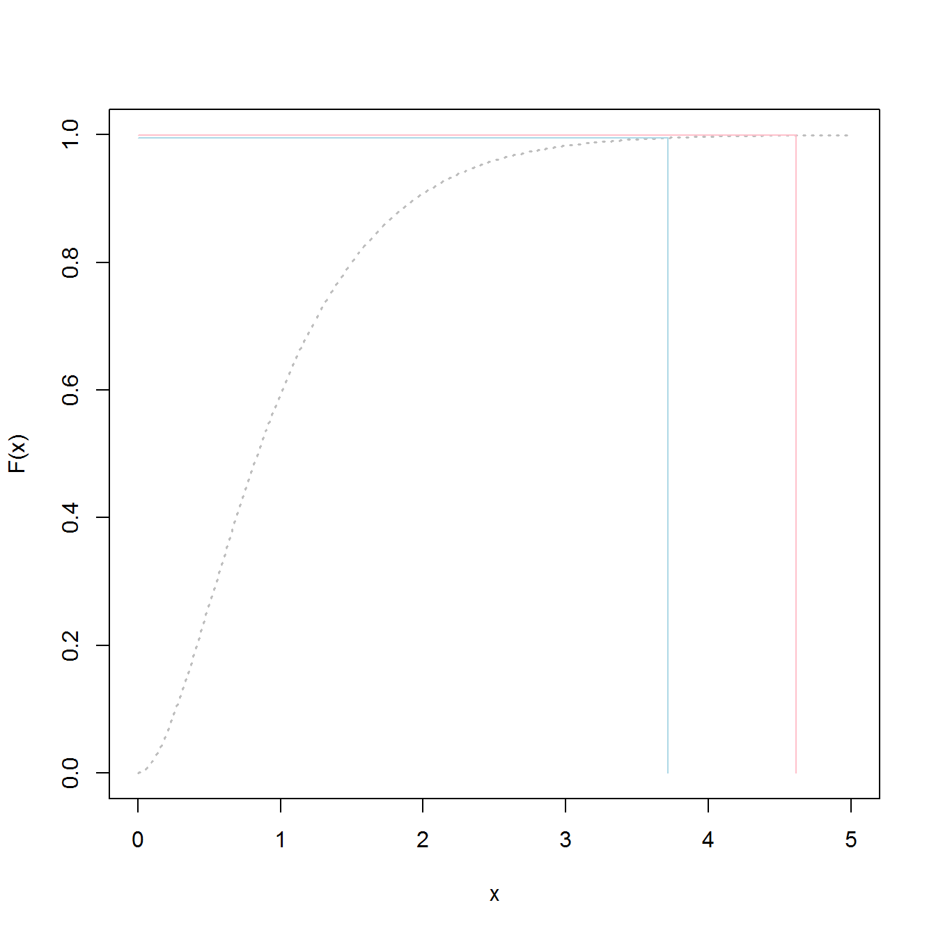
You might be thinking that the difference between 99.5% and 99.9% is minor; it's only 0.4% after all. But that's a difference in probability, and when you're in the tail, it can translate into a huge difference in quantiles. Here's an illustration of what it looks like for a gamma distribution, which doesn't have a very long tail as these things go. The blue line corresponds to the 99.5% quantile, and the red line is the 99.9% quantile. While the difference between these is tiny on the vertical axis, the separation on the horizontal axis is substantial. The separation only gets bigger for truly long-tailed distributions; the gamma is actually a fairly innocuous case.

enter image description here

$\endgroup$
8
  • $\begingroup$ Your answer is incorrect. The 99.9% point of a yearly Normal dies not correspond to a 1 in 1000 year event. The max of 1000 Normals has a different distribution. I think that's addressed in other answers. $\endgroup$ Commented Jul 5, 2015 at 23:59
  • $\begingroup$ @MarkL.Stone Nowhere did I say anything about the maximum of 1000 normals. $\endgroup$
    – Hong Ooi
    Commented Jul 6, 2015 at 0:13
  • 1
    $\begingroup$ That's exactly my point. The 1 in a 1000 years event should be based on the maximum of 1000 yearly Normal. That is very different than the 99.9$ point on a yearly Normal. See my comment to Karel Macek's answer below. $\endgroup$ Commented Jul 6, 2015 at 0:30
  • $\begingroup$ @MarkL.Stone The point of the graph is just to show that when you're in the tail, small changes in probabilities correspond to large changes in quantiles. You can substitute the 99% quantile of a GEV, or a GPD, or any other distribution. (And I didn't even mention the normal distribution.) $\endgroup$
    – Hong Ooi
    Commented Jul 6, 2015 at 0:35
  • $\begingroup$ Besides, estimating maxima via the GEV is just one way of getting tail quantiles. The other way is to estimate quantiles directly via the GPD (assuming a heavy-tailed distribution). $\endgroup$
    – Hong Ooi
    Commented Jul 6, 2015 at 0:37
6
$\begingroup$

Usually, the distribution of the underlying data (e.g., Gaussian wind speeds) is for a single sample point. The 98th percentile will tell you that for any randomly selected point there is a 2% chance of the value being bigger than the 98th percentile.

I'm not a civil engineer, but I'd imagine what you'd want to know is not the likelihood of the wind speed on any given day being above a certain number, but the distribution of the largest possible gust over, say, the course of the year. In that case, if the daily wind gust maximums are, say, exponentially distributed, then what you want is the distribution of the maximum wind gust over 365 days...this is what the extreme value distribution was meant to solve.

$\endgroup$
1
$\begingroup$

The use of the quantile makes the further calculation simpler. The civil engineers can substitute the value (wind speed, for instance) into their first-principle formulas and they obtain the behavior of the system for those extreme conditions that correspond to the 98.5% quantile.

The use of the whole distribution could seem to provide more information, but would complicate the calculations. However, it could allow the use of advanced risk-management approaches that would optimally balance the costs related to (i) the construction and (ii) the risk of the failure.

$\endgroup$
2
  • $\begingroup$ Well...I may not be clearly enough. I just want to know why use extreme value theory rather than the general distribution( the whole distribution? ) that we normally use? $\endgroup$
    – ZK Zhao
    Commented Jun 26, 2015 at 11:39
  • 1
    $\begingroup$ If the cumulative distribution function for any one instantiation, such as daily maximum wind speed, is F(x), then the cumulative distribution function for the maximum of n independent instantiations (e.g., n = 365 for a year's with of daily maximum wind speed) is F^n(x). This is different than F(x). $\endgroup$ Commented Jul 6, 2015 at 0:08

Your Answer

By clicking “Post Your Answer”, you agree to our terms of service and acknowledge you have read our privacy policy.

Not the answer you're looking for? Browse other questions tagged or ask your own question.