Extreme value distribution for multivariate normal

Question

I have a series of data sets. Each data set represents a measurement in 3D space relative to a global origin. I want to model the extreme values of my data. If I were to calculate the extreme radius and use that would I still expect a gumbel distribution? Alternatively I could produce a separate model for each axis if necessary but this is not as elegant as a single model. Ideally I would like to be able to predict the probability that a future experiment will have an extreme value less then X.

Is there anyway I can determine the parameters of the extreme value distribution from my normally distributed data? I have done some testing and it appears that I could reasonably assume that all my data sets are sample from the same population so I could assume this. Or, is it necessary to perform an MLE fit. I appreciate this functionality is available in most analysis software I was just curious how much one can tell about the properties of the EVD from the mean and standard deviation from which the extreme values are drawn.

Answer 1

Bowler, This is an interesting question that I see is unanswered. Memming suggested the Rayleigh distribution, which would work for two Axis (Plane) Radial errors Rxy Rxz Ryz from x,y,z Normally Distributed errors N(0,σ) (equal standard deviation's σ) for x, y, and z. The Radial error R=Sqrt(X N(0,σ)^2+ Y N(0,σ)^2) ~ Rayleigh(σ * Sqrt(2)). The Rayleigh is a special case of the Weibull with shape parameter (aka Slope) ß = 2. The Smallest Extreme Value Distribution (SEV) (Gumbel(min.)) is a location scale dist. related to the Weibull. The natural log of a Weibull random variable is a SEV. For example if X ~ Weibull(ß=2,Θ) ~ Rayleigh(Θ), then LN(X) ~ SEV(location LN(Θ),scale 1/ß = 0.5).

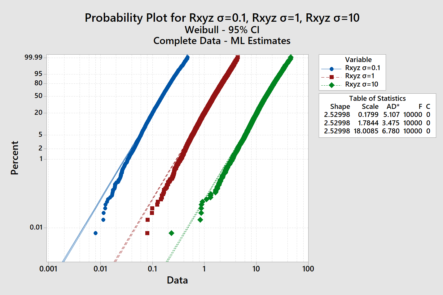
The 3D Radial error Rxyz from three x,y,z normally distributed errors each N(0,σ) would not be expected to be Rayleigh, but might be approximately Weibull. So, I ran an Monte Carlo and got the following Weibull Slope ß~2.53 (SEV Scale 0.395) Weibull Θ ~ 1.797 * σ (SEV Location ~LN(1.797* σ). The probability plot is curved, so it would only be a rough approximation. The Graph shows one of the three Monte Carlo Runs.

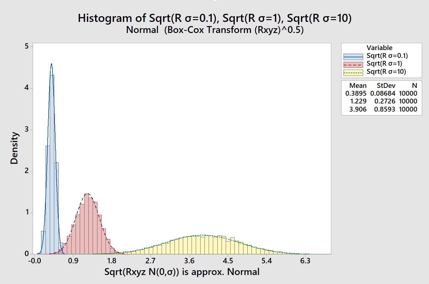
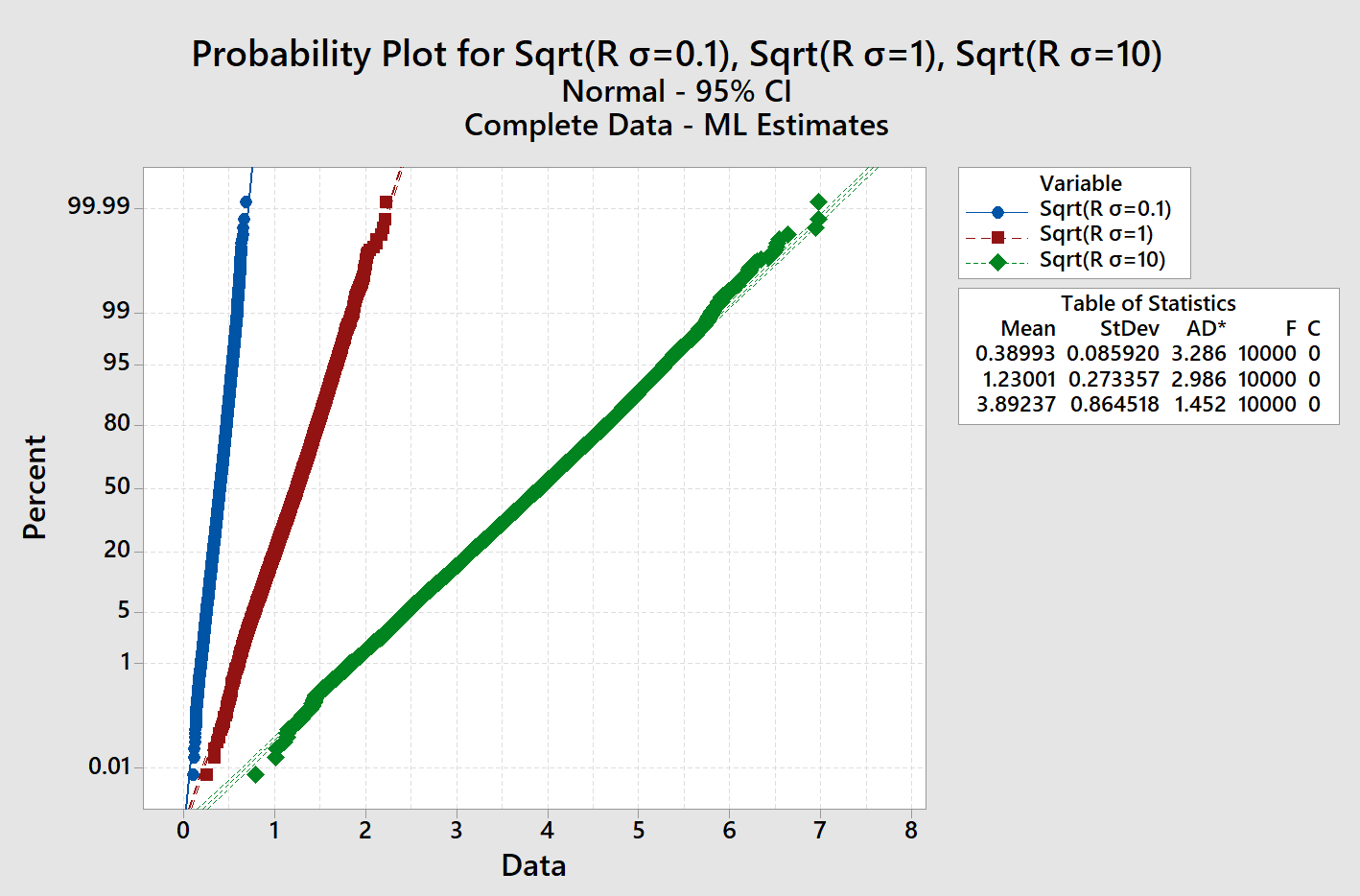
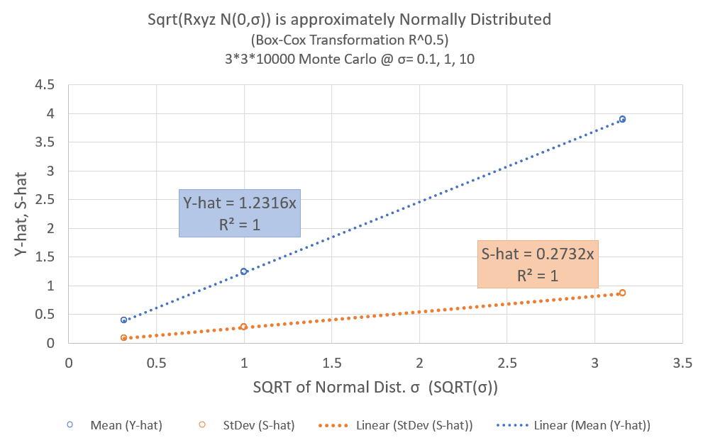
I also did a Box-Cox assessment since the Square Root of 2D Radial Error has been historically reasonably approximated by Rxy^0.5 (Sqrt(R)) being approximately Normally distributed. This resulted in a slightly better fit for these data, and the Sqrt(Rxyz) was near optimum for these data. In terms of being a function of the Normal Input Error σ for x,y,z. The relationship appears to be well modeled by a linear Y-hat, S-hat model for the Transformed Sqrt(Rx,y,z) as a function of the Square Root of the Normal Dist. Input Error σ. The Sqrt(Rxyz) Model ~ Normal(Y-hat,S-hat), where Y-hat = 1.2316* Sqrt(σ), S-hat = 0.02732 *Sqrt(σ). Normal Probability Plot for Sqrt(Rxyz) (one of three Monte Carlo runs). Y-Hat, S-Hat model. Bowler, I hope this helps...