14
$\begingroup$

I am reading Kevin Murphy's book: Machine Learning-A probabilistic Perspective. In the first chapter the author is explaining the curse of dimensionality and there is a part which i do not understand. As an example, the author states:

Consider the inputs are uniformly distributed along a D-dimensional unit cube. Suppose we estimate the density of class labels by growing a hyper cube around x until it contains the desired fraction $f$ of the data points. The expected edge length of this cube is $e_D(f) = f^{\frac{1}{D}}$.

It is the last formula that I cannot get my head around. it seems that if you want to cover say 10% of the points than the edge length should be 0.1 along each dimension? I know my reasoning is wrong but I cannot understand why.

$\endgroup$
1
  • 7
    $\begingroup$ Try picturing the situation in two dimensions first. If I have a 1m*1m sheet of paper, and I cut a 0.1m*0.1m square out of the bottom-left corner, I have not removed one-tenth of the paper, but only a hundredth. $\endgroup$ Commented Jun 28, 2015 at 23:43

4 Answers 4

14
$\begingroup$

That is precisely the unexpected behavior of distances in high dimensions. For 1 dimension, you have the interval [0, 1]. 10% of the points are in a segment of length 0.1. But what happens as the dimensionality of the feature space increases?

That expression is telling you that if you want to have that 10% of the points for 5 dimensions, you need to have a length for the cube of 0.63, in 10 dimensions of 0.79 and 0.98 for 100 dimensions.

As you see, for increasing dimensions you need to look further away to get the same amount of points. Even more, is telling you that most of the points are at the boundary of the cube as the number of dimensions increase. Which is unexpected.

$\endgroup$
5
$\begingroup$

I think the main thing to notice is that the expression

$$e_D(f) = f^{\frac{1}{D}}$$

is really really steep at the beginning. This means that the size of the edge that you will need to encompass a certain fraction of the volume will increase drastically, specially at the beginning. i.e. the edge you need will become ridiculously large as $D$ increases.

To make this even clearer, recall the plot that Murphy shows:
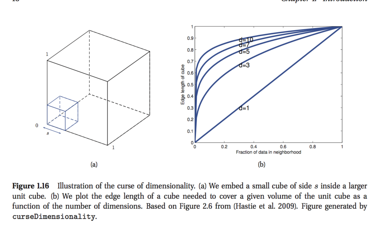
enter image description here

if you notice, for values of $D > 1$, the slope is really large and hence, the function grows really steeply at the beginning. This can be better appreciated if you take the derivative of $e_D(f)$:

$$ e'_D(f) = \frac{1}{D} f^{\frac{1}{D} - 1} = \frac{1}{D} f^{\frac{1 - D}{D}} $$

Since we are only considering increasing dimension (that are integer values), we only care for integer values of $D > 1$. This means that $1-D < 0$. Consider the expression for the edge as follows:

$$ e'_D(f) = \frac{1}{D} (f^{1 - D})^{\frac{1}{D}} $$

Notices that we are raising $f$ to a power less than 0 (i.e. negative). When we raise number to negative powers we are at some point doing a reciprocal (i.e. $x^{-1} = \frac{1}{x}$). Doing a reciprocal to a number that is already really small ( recall $f < 1$ since we are only considering fraction of the volume, since we are doing KNN, i.e. $k$ nearest data points out of the total $N$) means that number will "grows a lot". Therefore, we get the desired behavior, i.e. that as $D$ increases the power becomes even more negative and hence, the edge required grows a lot depending how large $D$ increases the exponent.

(notice that $f^{1 - D}$ grows exponentially compared to the division $\frac{1}{D}$ that quickly becomes insignificant).

$\endgroup$
2
$\begingroup$

Yeah, so if you have a unit cube, or in your case a unit line, and the data is uniformly distributed then you have to go a length of 0.1 to capture 10% of the data. Now as you increase the dimensions, D increases, which deceases the power and f being less than 1, will increase, such that if D goes to infinity the you have to capture all the cube, e=1.

$\endgroup$
2
$\begingroup$

I think for kNN distance plays a bigger role. As Bernhard Schölkopf put it, "a high-dimensional space is a lonely place". What happens to an (hyper) cube is analogous to what happens to the distance between points. As you increase the number of dimensions, the ratio between the closest distance to the average distance grows - this means that the nearest point is almost as far away as the average point, then it has only slightly more predictive power than the average point. This article explains it nicely

Joel Grus does a good job of describing this issue in Data Science from Scratch. In that book he calculates the average and minimum distances between two points in a dimension space as the number of dimensions increases. He calculated 10,000 distances between points, with the number of dimensions ranging from 0 to 100. He then proceeds to plot the average and minimum distance between two points, as well as the ratio of the closest distance to the average distance (Distance_Closest / Distance_Average).

In those plots, Joel showed that the ratio of the closest distance to the average distance increased from 0 at 0 dimensions, up to ~0.8 at 100 dimensions. And this shows the fundamental challenge of dimensionality when using the k-nearest neighbors algorithm; as the number of dimensions increases and the ratio of closest distance to average distance approaches 1 the predictive power of the algorithm decreases. If the nearest point is almost as far away as the average point, then it has only slightly more predictive power than the average point.

$\endgroup$

Your Answer

By clicking “Post Your Answer”, you agree to our terms of service and acknowledge you have read our privacy policy.

Not the answer you're looking for? Browse other questions tagged or ask your own question.